2.A.

Study Area

South Asia extends between 5°38^′39^″ and 36°54^′38^″ latitude and 61°05^′04^″ and 97°14^′12^″ longitude, with a land mass of 477 million hectares (Fig. 1, Table 1). The region lies within six agroecological zones: humid tropics, subhumid tropics, semiarid tropics, semiarid, subtropics, and arid.²⁰ Rice is grown within all these zones but is concentrated in the semiarid tropics and subhumid tropics. South Asia contains almost 200 million hectares of arable land area. Water supply is either from irrigation (∼80 million hectares, where water is supplied via canals, water tanks, or groundwater) or rainfall (∼120 million hectares).²¹ Figure 1 shows the major drainage basins in South Asia and the command areas where irrigation is present in India.

Rice cropping occurs in three seasons across the region: the main kharif or aman during the monsoon (June to mid-December), the rabi or boro in the postmonsoon dry season (mid-December to March), and a summer-season aus crop (April and May). Rice is harvested on some 60 million hectares across all three seasons (Table 1). Irrigated areas include double cropping of rice and other grains, single cropping of sugarcane, chilli, cotton, fodder grass, and some areas of light irrigation of corn, sorghum, and sunflower. Rain-fed crops include grains (sorghum, millet), pulses (red gram, green gram, and chickpea), and oilseeds (sunflower and groundnut).

2.B.

MODIS Data Preprocessing

2.C.

Field-Plot Data for Identifying, Labeling, and Assessing the Accuracy of MODIS-Based Rice Maps

Field-plot data were collected during October 11–26, 2003, and August 30–September 28, 2005. Interviews with farmers and agricultural extension officers were conducted to determine cropping types and conditions, including the collection of historical data as far back as 2000 to 2001. A total of 1004 locations covering the major crop-land areas (Fig. 2) were chosen based on the knowledge of local agricultural extension officers to ensure that adequate samples of rice as well as other crops were gathered. The local experts also provided information on crop calendars, cropping intensity (single or double crop), and percentage canopy cover for these locations. Of the 1004 data points, 75% (751) were used for class identification and calculating rice fractions (within this, 149 rice points were used for ideal temporal profile generation) and the rest of the points (253) were used for the following accuracy assessment.

Fig. 2

Field-plot data-point locations in South Asia. There are 1004 field-plot locations where crop type, cropping intensity, watering source (irrigated versus rainfed), and a number of other parameters (e.g., digital photos, land cover distribution) were also collected.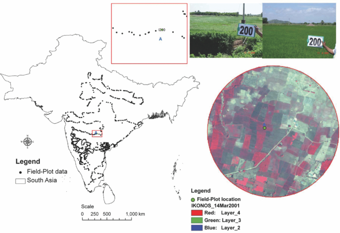

The precise locations of the sample sites were recorded using a Garmin handheld global positioning system unit. Ideally, 50 or more samples should be collected per land use class,²³ but, due to limited resources, the sample size varied from 15 to 25 for each major crop-land use/land cover (LULC) class.

At each of the 1004 locations, the following data were recorded for 2000 to 2001 based on interviews with local agricultural extension officers and/or farmers:

These class labels were assigned in the field, but additional class information was incorporated later on the basis of visual interpretation of the LandSat GEOCOVER 2000 data set.²⁴ Most of the Google Earth images were very high resolution (submeter to 4 m; from IKONOS, Quickbird satellites, and Landsat images) and were acquired in recent years. These data again relate to the target mapping for the 2000 to 2001 season.

2.D.

Ancillary Spatial and Statistical Data

Several ancillary (or secondary) spatial data sets were used to segment the MODIS data into various components in order to augment the classification procedure and increase the accuracy in identifying rice classes.

2.D.2.

Irrigation command areas to segment them from the rest of the areas

Irrigated command areas are a clear indication of where surface (canal)-irrigated crops are cultivated. We obtained irrigated command area maps from India and used them to further split the ≤2% slope gradient segment into irrigated and nonirrigated areas (Fig. 3). Crop lands within these command areas are almost always irrigated (with the possible exception of more remote areas during drought periods). Naturally, there are always some LULC classes within the command area segment that are not crop land, but the command area segment will still aid classification accuracy with respect to irrigated rice areas.

Fig. 3

Methodology overview. Overview of the methodology for mapping rice areas using the eight-day MODIS MOD09A1 data and other ancillary spatial data. There were six image segments of a MFDC.

3.1.

Overview of Methods

An overview of the methods is shown in Fig. 3, and each step is described in detail in this section.

The process starts with the conversion of the MODIS data into GeoTIFF format, the removal of clouds as documented in Ref. 16, and the generation of MFDCs (see Ref. 17 for a detailed description), in which the multispectral time-series data are combined into a single-file data cube involving numerous data layers (see also Sec. 4.1.3). The MODIS MFDC is divided into distinct segments (see Secs. 3.3.1–3.3.3) to allow for easier class spectrum separation and class identification.

3.2.

Ideal Temporal Profile (Normalized-Difference Vegetation Index Curves) Creation

The rice and nonrice fields were located exactly on the South Asia image (Fig. 4). The 149 rice points represent distinct categories of rice (e.g., double crop, single crop). The sample sizes of each category are indicated within the brackets of class legend in Fig. 5. The temporal profile signatures (e.g., NDVI, reflectivity) gathered for the 149 rice fields were grouped according to their unique categories and a typical ideal temporal profile (Fig. 5) of that particular category of rice crop established. When there were classes within classes (e.g., when an irrigated-rice-double crop has distinctly different signatures because of, say, cropping calendars), then we have two ideal temporal profiles for this class. This resulted in an ideal temporal profile of 12 distinct rice classes (Fig. 5) aggregated from the 149 sample locations.

Fig. 4

Phenology of the rice crop. Typical phenologies of six types of rice crops (e.g., double crop, single crop) of South Asia illustrated using NDVI signatures of MODIS time series. Top image is a false color-composite image of South Asia based on MODIS bands 1, 2, and 4 from October 31, 2000.

Fig. 5

Ideal temporal signatures (NDVI curves) for the 12 rice classes. The ideal temporal profiles of 12 rice classes were generated using MODIS time-series data. Note: Field-plot sample size is shown in brackets (“sw” is surface water; “gw” is groundwater, “sc” is single crop, and “dc” is double crop).

3.3.

Class Temporal Profile (Normalized-Difference Vegetation Index Curves) Generation

The MFDC was divided into five distinct segments (see Fig. 3) based on elevation, slope, water bodies, and command areas. The first set of segments was (a) water-body segment, (b) elevation segment 1: >2500 m, and (c) elevation segment 2: ≤2500 m. Segment c was further divided into three subsegments, which were c1 slope segment 1: >2% gradient, c2 slope segment 2: ≤2% gradient, and c3 irrigation command area. The main aim of the segmentation process was to focus more on the segments having higher amounts of crop-land classes such as the Central Board of Irrigation and Power (CBIP) command areas (e.g., India), valley bottoms, deltas, and river banks.

Unsupervised classification using the ISOCLASS cluster classification^{17, 18} (ISODATA in ERDAS Imagine 9.2^™)³³ was applied to each of the MFDC segments. The classification was set at a maximum of 100 iterations and a convergence threshold of 0.99. In this study, the number of classes varied from 20 to 100 based on area spreading and complexity of segment. Segment 1 (elevation >2500 m) was classified into 20 classes because of lower complexity, and most of the areas are forested, snow-/ice-covered, or barren. Slope segments 1 and 2 were classified into 50 classes each, whereas the irrigation command area segment, which covered a larger and more complex area (with a mix of irrigated crops, irrigated dry crops, and rain-fed crops), contained 100 initial classes, making a total of 220 classes across all segments.

Class temporal profiles were generated using ISOCLASS k-means classification of each of the segment MFDCs. Each segment was classified into 100 classes. The signature file of the 100 classes was plotted, and similar classes were then grouped [e.g., Fig. 6b illustrates a few of the class temporal profiles]. The process of matching class temporal profile [e.g., Fig. 6b] with ideal temporal profile [e.g., Fig. 6a] is illustrated in Figs. 6c, 6d. The process is repeated for other groups of classes, until all classes are resolved. The class temporal profiles that do not have a match with any ideal temporal profile are resolved using other approaches (e.g., Secs. 3.4 and 3.5). The quantitative approaches of SMTs are described in detail by Ref. 19. The process is repeated for classes from all segments.

Fig. 6

Decision-tree algorithm. The classes were also grouped and identified using the NDVI-based decision-tree algorithms. Note: Illustrated here for segment c3 classes. Each plot is NDVI (y) versus time (x).

3.4.

Decision-Tree Algorithms

Several techniques were used simultaneously to group the classes in each segment. The first reduction in classes used a decision tree³⁴ based on the temporal NDVI MVC data. The decision tree is based on NDVI thresholds at different stages in the season that define the vegetation growth cycle, and these algorithms help to identify similar classes. The dates and threshold values were derived from the ideal temporal profile. The decision tree for segment c3 is shown in Fig. 7. This first stage reduced the total number of classes from 220 to 127.

Fig. 7

Spectral matching technique (SMT). In SMTs, the class temporal profiles (NDVI curves) are matched with ideal temporal profiles (quantitatively based on temporal profile similarity values) in order to group and identify classes as illustrated for a rice class in this figure. (a) Ideal temporal profile illustrated for “irrigated-surface-water-rice-double crop”; (b) some of the class temporal profile signatures that are similar, (c) ideal temporal profile signature [Fig. 7a] matched with class temporal profiles [Fig. 7b], and (d) the ideal temporal profile [Fig. 7a, in deep green] matches with class temporal profiles of classes 17 and 33 perfectly. Then one can label classes 17 and 33 to be the same as the ideal temporal profile (“irrigated-surface-water-rice-double crop”). This is a qualitative illustration of SMTs. For quantitative methods, see Ref. 29.

The second and subsequent groupings used spectral matching techniques (SMT),^{17, 18} such as those used for hyperspectral analysis of minerals (e.g., Refs. 19, 34, and 35). Time-series data, such as the eight-day MODIS NDVI data, are similar to such hyperspectral data with the 327 bands stacking a single instance of a hyperspectral image (or monthly NDVI values). These similarities imply that the SMTs applied for hyperspectral image analysis also have potential for application in identifying agricultural land-use classes from multiband time-series satellite imagery.

The temporal profile signatures of the classes within each segment were further grouped based on temporal profile similarity and compared against the ideal temporal profile in order to identify and label the grouped classes (Fig. 6). Additionally, we used the field-plot data points, imagery from Google Earth and GeoCover, as well as national statistical data as auxiliary data in the class labeling. On the basis of one or more of these data, we clearly established that irrigated crop lands have distinct phenological cycles compared to rain-fed crop lands. For example, irrigated crops are often planted later than rain-fed crop lands, have a longer phenological cycle, and often have a following crop. All these factors are monitored using the MODIS time series. However, it must be noted that the magnitude of NDVI is not an indicator in distinguishing between rain-fed and irrigated crops, because we found that, in some cases, rain-fed crops actually have a higher magnitude of NDVI than irrigated crops. This may happen, for example, in flood-irrigated crops, for which background water can substantially absorb near-infrared reflectivity, thus reducing NDVI. Two main properties of class signatures allow the separation of groundwater and surface-water irrigation: annual average NDVI, which is a function of the irrigated fraction, and timing of the onset of greenness, which is a function of the timing of water availability for vegetation. Annual NDVI in both continuous and double-irrigated systems exceeds annual NDVI in groundwater systems, reflecting the higher irrigated fraction in areas irrigated with surface water. An example of spectral matching is shown in Fig. 6 for the irrigated-surface-water-rice-double crop.

3.5.

Resolving Mixed Classes

A rigorous class-identification and labeling process (Sec. 3.4) helped in identifying, grouping, and labeling many classes. However, some complex classes remained unresolved as mixed, because the purity of these classes could not be adequately validated using field-plot data and/or very high-resolution imagery, and/or other means. The mixed classes have more than one class in them. When classes continued to be mixed, in spite of the various methods and techniques discussed in previous sections, we adopted GIS spatial modeling approaches to resolve the classes. This involved taking mixed classes and applying spatial modeling techniques, such as overlay, matrix, and recode,³³ based on the theory of map algebra and Boolean logic.^{36, 37, 38} The spatial data layers used included elevation zones and rainfall zones. Any one or a combination of these data layers usually helped in separating the mixed classes. For example, when some other agricultural areas mixed with rice classes, we ran a matrix with elevation classes as one axis of the matrix and a mixed class as the other axis to obtain classes at different elevation gradients. In such a scenario, we separate the mixed class into various elevation zones and rice may be one of these classes. Similarly, we can use elevation with precipitation as one of the axes of the matrix. All these different possibilities were attempted until the mixed class got resolved.

Furthermore, a rule-based decision-tree algorithm was used to help split the mixed classes. One sample application used NDVI variations in specific months in different parts of the same class to separate the classes. Whenever spatial modeling and decision-tree algorithms were unsuccessful, the mixed classes were masked out and the MFDC covering this area was used to reclassify the image into a number of classes. This was followed by a repetition of the entire class-identification and labeling process.

In spite of the rigorous class-identification process described in these sections, there were still some mixed classes. Typically, the unresolved classes were then split up into 5–10 or more subclasses (depending on the extent of area and complexity), reclassified using the masked area of the megafile data cube and the class-identification and labeling process (as described previously), and repeated.

3.6.

Actual or Subpixel Area Calculations

The composite MODIS pixels cover an area of 21.5 hectares, which is larger than many agricultural fields in the study area. Thus, many pixels contain more than one land-cover class (Table 3). Any rice classification derived from such data will provide only the full pixel area (FPA), whereas the actual rice area per pixel can be obtained only by computing subpixel areas (SPAs) [Eq. 3],^{17, 19, 39} which are defined as

Table 3

Rice classes (irrigated and rain-fed) mapped in this study. The table shows FPA, rice-area fraction (RAF), and SPA or actual area. SPA = FPA × RAF. Note: 12-class map in Fig. 8, signatures in Fig. 9.

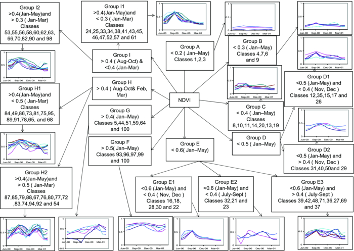
4.A.

Classification Assessment Based on Field-Plot Data

A fuzzy accuracy assessment (Table 4) was performed using 25% (251 data points out of 1004) of the field-plot data to derive a robust understanding of the accuracies of the data sets used in this study. The field-plot data were based on an extensive field campaign conducted throughout India during kharif and rabi seasons by International Water Management Institute researchers, and they consisted of 1004 points. About 30% of the points were collected during the rabi season.

Table 4

Fuzzy accuracy assessment from field-plot data. Values in the table indicate the percent of field-plot windows in each class with a given correctness percentage.

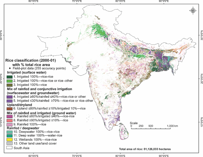
Fuzzy accuracy assessment provides realistic class accuracies for which land cover is heterogeneous and pixel sizes exceed the size of uniform land cover units (see Refs. 16, 17, 39, and 40). For this study, we had assigned 3 × 3 cells of MODIS pixels around each of the field-plot points to one of six categories: absolutely correct (100% correct), largely correct (75% or more correct), correct (50% or more correct), incorrect (50% or more incorrect), mostly incorrect (75% or more incorrect), and absolutely incorrect (100% incorrect). Class areas were tabulated for a 3 × 3-pixel (nine-pixel) window around each field-plot point.

On the basis of the theoretical description given by Ref. 23, Eqs. 4, 5, 6 were used to estimate accuracies and errors. Field-plot information was used to determine robust accuracies, using Eqs. 4, 5, 6,

4.B.

Accuracy Assessment Based on Correlations between Census-Derived Rice Areas versus MODIS-Derived Rice Areas

The field-plot data points were used to compute fractional rice areas for each rice class, that is, the proportion of the “rice” MODIS pixel that was planted to rice, and this in turn was multiplied by the number of MODIS rice pixels per subnational unit to derive a physical rice area estimate to compare to published rice area statistics. This combined the strengths of both “accuracy-assessment” approaches. We performed the comparison at the regional, national, state, and district levels.

5.A.

Rice Map and Area Statistics

Altogether, 12 rice classes were identified and labeled (Fig. 8). The final class name or label (Fig. 8, Table 3) is based on the predominance of a particular rice class (e.g., single- or double-season rice), and the dominant water source (e.g., irrigated or rain-fed). For example, the name for class 1 is “01. Irrigated 100 percent—rice-rice (meaning first-season rice followed by a second rice crop).” This means that rice class is dominated by rice cultivation in both the kharif and rabi seasons, and the area is predominantly irrigated from surface-water sources. This class occurs in the major command areas such as the Ganges, Indus, and Krishna. Similarly, class 9 is labeled “09. Rain-fed 100 percent—rice” because this is an intensely cropped rice class, but heavily dependent on seasonal rains. This class is predominantly found in heavy-rainfall areas such as those in Sri Lanka and some parts of eastern and southern India. Similarly, class 2 is labeled “02. Irrigated 100 percent—rice-rice or rice-other crop,” found predominantly in the Indo-Ganges basin command areas and Godavari delta. Class 3 is called “03. Irrigated 100 percent—rice,” occurring primarily across Orissa, Chhattisgarh, and fragmented areas in Uttar Pradesh in India and across Pakistan. Classes 4 and 5, “irrigated/rainfed rice areas,” predominate in Tamil Nadu and Bangladesh. Class 6 is “06.Upland ≥80 percent/rain-fed ≤10 percent/irrigated ≤10 percent—rice” areas, which are found primarily in Madhya Pradesh, Maharashtra, and fragmented locations across the study areas. Classes 10 and 11 (“Deepwater 100 percent rice-rice” and “Deepwater 100 percent water-rice”) and Class 12 (“Wetlands 100 percent rice-rice”) are predominant in Bangladesh and fragmented areas along the coastal regions (Fig. 8, Table 3). The spectral separability in the temporal NDVI signatures for each of the rice classes is shown in Fig. 9.

Fig. 8

The 12 rice classes of six South Asian countries mapped based on MODIS 500-m seven-band time-series data for 2000 to 2001. Note: Area statistics of these classes in Table 3, signatures in Fig. 9.

Fig. 9

The temporal mean MODIS 500-m NDVI signatures of the 12 rice classes derived using data for 2000 to 2001. Note: The 12-class map is in Fig. 8 and area statistics in Table 3.

5.B.

Vegetation Phenology of Various Rice Classes

Rice-crop phenology was studied using NDVI time-series plots (Fig. 9). These NDVI time-series profiles provided information on (Fig. 8): (i) cropping intensities (e.g., single or double crop); (ii) crop calendar (i.e., when a crop begins and when it is harvested); and (iii) crop health and vigor (indicated by magnitude of NDVI). Each rice class (Fig. 8) has a distinctly different phenology depicted by the NDVI magnitude and/or seasonality (Fig. 9).

The NDVI time series also allows the separation of rain-fed rice from irrigated rice based on factors such as when a crop calendar begins and the magnitude of NDVI. For example, class 2 (Fig. 9) shows a kharif crop beginning around June 20, NDVI peaking around August 15, and the crop harvested by the end of October. The rabi crop begins around November 15, NDVI peaks around February 15, and all crops are harvested by April 15. Around October 15 (Fig. 9), this class 2 has the lowest NDVI and a uniquely high NDVI (compared to all other classes) around December 15. Such distinctive features indicate a unique class with a firm set of characteristics that define that class. This can be said of all classes depicted in Fig. 9.

5.C.

Rice Area Fractions

Each rice class has several different land cover classes (Fig. 9, Table 3); however, all 12 rice classes have more than a 90% rice-area fraction (RAF) (Table 3). Thus, all 12 rice classes are relatively pure rice classes. However, when calculating actual rice areas (or subpixel areas), we should use RAFs. For example, in class 2 (02. Irrigated 100 percent—rice/rice or rice/other), rice areas (90.3%; Table 3) dominate, but there are other land-cover types, including 1.1% trees, 0.3% shrubs, 1.3% grass, 0.4% built-up area, 2.7% water, and 3.8% other crops (Table 3).

Therefore, the actual areas or SPAs of class 2 in Table 3 = 8,999,360 hectares of FPAs × (93.3/100 of RAFs) = 8,127,089 hectares. Using the same approach, the actual areas (SPAs) of the other 11 rice classes are calculated (Table 3).

5.D.

Accuracy Assessment

The classification accuracies obtained from the 268 independent field-plot observation data points (15 extracted from other secondary sources and high-resolution images) are summarized in Table 4. The fuzzy classification accuracy varied between 67% and 100% across 12 classes, with an overall accuracy of 80%. However, it must be noted that most rice classes intermix among themselves. Thus, the uncertainty of ∼20% is due to the intermixing among the various rice classes. Thus, rice versus no-rice class accuracy will be very high. The irrigated classes generally have higher classification accuracies than the rain-fed or mixed irrigated/rain-fed classes (Table 4).

5.E.

Accuracy Assessment Based on Comparison to Subnational Statistics and Other Published Rice-Area Estimates

Table 5 compares the summed RAFs across all classes against the published rice statistics by the six countries. The comparison at the district level (812 spatial units) was performed across South Asia, but, for reasons of space, we report only the tabulated areas at the state level (54 spatial units), and the district-level comparison is shown in Fig. 10. Figure 10 shows the relationship between the MODIS area summarized at district and state levels and the subnational rice areas at the same level of spatial detail. The level of agreement between the MODIS area estimates and the published statistics is very good, 97% at the district level [Fig. 10a] and 99% at the state level [Fig. 10b]. This excellent match between MODIS-derived rice areas and national and subnational statistics clearly illustrates the high accuracy with which MODIS data have been classified.

Fig. 10

Rice areas of South Asia derived using MODIS 500 m compared to agricultural census data for 2000 to 2001: (a) district-wise and (b) state-wise (below). (Administrative boundaries are shown in Fig. 1.)

Table 5

Comparison of MODIS rice area estimates with subnational statistics, by state.

These rice maps and statistics produced in this study were a clear advancement over the early rice maps^{9, 10, 11} in which remote-sensing data were not used. Those early maps were produced by putting together maps and statistics of varying scales and accuracies obtained from different countries and regions using distinctly different approaches to mapping.^{9, 10, 11} Later rice maps^{6, 12, 13, 14} used remote sensing and were vast improvements over earlier^{9, 10, 11} maps. However, these later efforts used a single methodological approach (e.g., vegetation indices as in Ref. 6) that left considerable uncertainties.^{5, 15} As a result, this study used not only multitemporal remote sensing from MODIS but also a suite of methods to decrease uncertainties and achieve a high degree of accuracy in spatial maps and/or statistics derived from them.