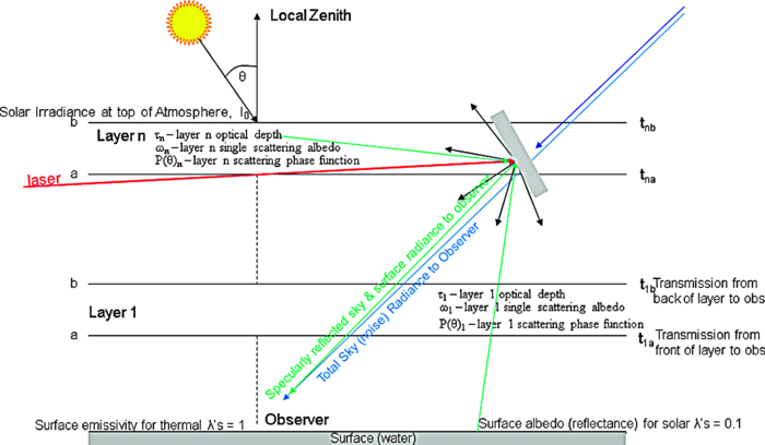
1.

Introduction

One of the primary factors affecting the analysis and processing of multi-, hyper-, and ultraspectral sensor data is correcting or compensating for the wavelength-dependent atmospheric effects on the various parts of the spectrum considered. The Air Force Institute of Technology Center for Directed Energy (AFIT/CDE) has developed several modeling codes that are unique in the manner and sophistication in which they characterize atmospheric parameters as they affect the propagation of electromagnetic radiation. By analyzing the expected high spectral resolution characteristics of electromagnetic propagation with broadband modeling tools, AFIT/CDE is able to assess the expected response of sensors designed to monitor the interaction of delivered energy with materials at the terminus of the beam. This paper presents an example of a high fidelity simulation of a bistatic, time-varying five band multispectral remote observation of energy delivered on a distant and receding test object. AFIT/CDE's Remote Observer Scenario Toolkit predicts remotely sensed, time-varying radiance arising from such a test object for any location worldwide, time of day, any collection geometry, and any combination of spectral bands. Such spectral data are useful in developing and evaluating algorithms for remotely assessing temporally and spatially evolving irradiance on the test object's surface.

In order to fulfill its technical objectives, AFIT/CDE developed the Remote Observer Scenario Toolkit to simulate a wide range of test object signatures and sensor performance for any focal plane design and for any combination of wavelength bands of any spectral width from the visible to the longwave infrared (LWIR). An extremely wide range of worldwide atmospheric effects are available to include path transmittance, path radiance, earthshine, and skyshine contributions to the signal level. The model features true three-dimensional (3D) geometry on a spherical earth, and supports any relationship between the platform, test object, observer location, and solar position. The faceted test object may have any orientation and, in combination with a spectrally and temperature dependent bidirectional reflectance distribution function (BRDF), is available for several materials, and allows accurate calculation of reflected and emitted energy in any direction. The faceted test object may be defined to have any shape; in the current example it is cylindrical. Any BRDF model can be used in the simulation, given the availability of material-specific parameters for that model. The typical platform-target-observer geometry modeled in the Remote Observer Scenario Toolkit is depicted in Fig. 1.

Fig. 1

Irradiance and imagery measurements engagement geometry.

A detailed description of the Remote Observer Scenario Toolkit and its various component models, to include computational codes, propagation codes, atmospheric models, target interaction models, BRDF algorithms, and sensor models, follows in Sec. 2. Section 3 provides results and discussion of the example simulation. Section 4 is a summary with conclusions.

2.

Remote Observer Scenario Toolkit Description

AFIT/CDE's Remote Observer Scenario Toolkit is based on, and leverages, established directed energy community tools and legacy imaging model tools. These tools include the High Energy Laser End to End Operational Simulation (HELEEOS).¹ AFIT/CDE developed the HELEEOS model, under the sponsorship of the High Energy Laser Joint Technology Office, in part to quantify the performance variance created by the natural environment in possible laser engagements. As such, HELEEOS includes a fast-calculating, first principles atmospheric propagation and characterization package. This package enables the creation of profiles of temperature, pressure, water vapor content, optical turbulence, and atmospheric particulates and hydrometeors as they relate to line-by-line layer extinction coefficient magnitude at wavelengths from the ultraviolet to radio frequencies. Sensor model concepts from the Hyperspectral Sensor Image Model² and the Image Based Sensor Model³ were also incorporated in the Remote Observer Scenario Toolkit. A realistic and accurate prediction of the potentially temporally evolving irradiance pattern on the test object is the critical initial step in the Remote Observer Scenario Toolkit chain, and can be provided by HELEEOS in conjunction with another community tool, the Scaling for High Energy Laser and Relay Engagement (SHaRE) toolbox.⁴ Delivered irradiance depends on outgoing laser power, platform adaptive optics, atmospheric effects, engagement velocities, and engagement geometry. Realistic test object kinematics can be computed using any appropriate model.

Though considerable information regarding energy deposited can be obtained from the in-band diffuse reflection from the test object, thermal radiation data arising from the hot spot can reduce uncertainty in any subsequent irradiance estimate. Delivered irradiance-test object interaction modeling was added to the Remote Observer Scenario Toolkit to obtain thermal radiation intensities from the resulting hot spot on the test article. Delivered irradiance interaction with the test object is modeled primarily in ABAQUS. ABAQUS is a suite of powerful engineering simulation programs that are based on the finite element method.⁵ Extensive research was conducted during the current study on realistic wavelength and temperature-dependent BRDFs for several common materials to provide an accurate time resolved prediction of the hot spot's spectral radiance. A schematic of the inputs required, the models used, and the results obtained in the CDE Remote Observer Toolkit are shown in Fig. 2.

Fig. 2

Schematic of the CDE Remote Observer Scenario Toolkit.

2.A.

Atmospheric Effects

The HELEEOS model enables the evaluation of variability in high energy laser propagation by incorporating probabilistic climatological data on the parameters that drive most major atmospheric effects. The atmospheric parameters investigated, such as temperature, pressure, water vapor content, optical turbulence, and atmospheric particulates, are put into vertical profiles of data for highly specific modeling scenarios. The worldwide seasonal, diurnal, and geographically varying databases, covering all land and ocean regions underlying the HELEEOS atmospheric model, have been described in earlier publications,^{1, 6, 7} and are available in a stand-alone atmospheric characterization software code called the Laser Environmental Effects Definition and Reference (LEEDR).⁸

For the Remote Observer Scenario Toolkit, AFIT/CDE incorporates a single scattering path radiance calculation capability into the HELEEOS atmospheric computational engine. This greatly simplifies the inclusion of path radiances into the engagement scenarios, and allows the full utilization of the HELEEOS atmospheric characterizations in the radiance calculations. The techniques employed to calculate the single scattered sky, path, and background radiances adhere closely to those described in documentation for MODTRAN.^{9, 10} The primary difference from the MODTRAN calculations is that radiative transfer in HELEEOS is computed line-by-line rather than at moderate resolution broadband. The technique used in MODTRAN is actually more relevant in the HELEEOS and Remote Observer Scenario Toolkit application as Beer's Law extinction is exact for monochromatic radiative transfer.

Radiance into an observation path comes primarily from two sources: surface and atmospheric emissions in the infrared and scattered ultraviolet to near-infrared (NIR) energy from the Sun or other celestial objects. Emissions from the sky and the surface are often referred to as the “thermal” or “longwave” component of path radiance, and the solar radiation is typically called the “shortwave” component. Both components are reflected/scattered by the earth's surface and by atmospheric particulates such as aerosols, water and ice cloud particles, and precipitation. Rayleigh scattering caused by air molecules is significant at shorter wavelengths (below 1 μm), and is an important consideration for solar scattering and laser propagation. HELEEOS models the single scattered solar radiation by accounting for the top-of-the-atmosphere solar spectrum, the curvature of the earth, and engagement-specific distribution scattering phase functions based on Rayleigh and Mie theory.¹⁰

Figure 3 is a schematic depiction of the radiative transfer geometry for the Remote Observer Scenario Toolkit. North is on the right side of the schematic, south on the left. The relationships among the high energy laser (HEL) radiation, the background radiance, the total sky radiance, and the specular and diffuse reflections off the test object are graphically shown in Fig. 3. The atmosphere is broken into “n” number of layers (∼100) from the surface to the top of the HELEEOS atmospheric definition—100 km. All calculations are done for each layer and all nonvertical path lengths are accounted for before integrating (summing) over the path lengths. The earth's surface is considered as a separate source layer in the integration—as an emitter of thermal radiation and a scatterer/reflector at solar wavelengths. The emissivity of the assumed ocean surface is set at 1.0 for thermal wavelengths and the albedo is set at 0.1 for solar wavelengths.

Fig. 3

Schematic of the radiative transfer geometry in the Remote Observer Scenario Toolkit.

Path transmittance (unitless), t, is calculated monochromatically via Beer's law and the plane-parallel assumption:

Eq. 1

[TeX:] \documentclass[12pt]{minimal}\begin{document}\begin{equation} t(z_1,z_2) = e^{ - \tau (z_1,z_2)/\left| {\cos \theta } \right|} \end{equation}\end{document} $t(z_1,z_2)=e^{-\tau (z_1,z_2)/\left|\cos \theta \right|}$

where τ is the optical depth (unitless), z is the geometric height (m), and β_e is the volume extinction coefficient (m⁻¹) as shown in Eq. 2.

Eq. 2

[TeX:] \documentclass[12pt]{minimal}\begin{document}\begin{equation} \tau (z_1,z_2) = \int_{z_1 }^{z_2 } {\beta _e (z)dz}. \end{equation}\end{document} $\tau (z_1,z_2)={\int }_{z_1}^{z_2}{\beta }_e\left(z\right)dz.$

Total single scattering spectral path radiance (W cm⁻² sr⁻¹ μm⁻¹) is calculated in a manner similar to MODTRAN.¹⁰ HELEEOS, and its atmospheric characterization code LEEDR, first define the atmosphere in a user specified number of layer slabs based on the vertical profile conditions for the site, time of season, time of day, surface visibility, and boundary layer height of interest. The path radiance contribution of a slab with lower and upper boundaries a (nearer to the observer) and b (farther from the observer, as shown in Fig. 3) is given by:

Eq. 3

[TeX:] \documentclass[12pt]{minimal}\begin{document}\begin{equation} I_{\lambda,{\rm path}} = \int_{t_b }^{t_a } {Jdt = } \overline J \left( {t_a - t_b } \right) = t_a \overline J \left( {1 - t_L } \right) = t_a \int_{t_L }^1 {Jdt} \end{equation}\end{document} $I_{\lambda ,\mathrm{path}}={\int }_{t_b}^{t_a}Jdt=\overline{J}\left(t_a-t_b\right)=t_a\overline{J}\left(1-t_L\right)=t_a{\int }_{t_L}^{1}Jdt$

where t_a and t_b are transmittances from the observer to the slab a and b boundaries along the line of sight (LOS), t_L is the transmittance of the slab, and the integration is along the LOS. For HELEEOS and LEEDR, J is the total source term including the single scattering solar and thermal components. The term t_a is the foreground transmittance from the observer to the front of the layer, and [TeX:] $\overline J$ $\overline{J}$ (1-t_L) is the “self-radiance”¹⁰ of the layer slab. Thus the path radiance, without additions for surface terms, is the sum of the self-radiance of each layer slab weighted by the radiance between the slab and the observing sensor. For up-looking scenarios like that depicted in Fig. 3, the total source, J (W cm⁻² sr⁻¹ μm⁻¹), consists of two terms as shown below for the self-radiance of layer L:¹⁰

Eq. 4

[TeX:] \documentclass[12pt]{minimal}\begin{document}\begin{equation} \int_{t_L }^1 {Jdt} = J_{{\rm thermal}} + J_{{\rm sss}}. \end{equation}\end{document} ${\int }_{t_L}^{1}Jdt=J_{\mathrm{thermal}}+J_{\mathrm{sss}}.$

The thermal source term (W cm⁻² sr⁻¹ μm⁻¹) is computed via the following:

Eq. 5

[TeX:] \documentclass[12pt]{minimal}\begin{document}\begin{equation} J_{{\rm thermal}} = \left( {1 - \omega _L } \right)\int_{t_L }^1 {L_\lambda (T)dt} = \sum_{t_L }^1 {\left( {1 - \omega _L } \right)\left\{ {L_\lambda (T)\left[ {1 - t_L } \right]} \right\}}, \end{equation}\end{document} $J_{\mathrm{thermal}}=\left(1-{\omega }_L\right){\int }_{t_L}^1{L}_{\lambda }\left(T\right)dt=\sum _{t_L}^1\left(1-{\omega }_L\right)\left\{L_{\lambda }\left(T\right)\left[1-t_L\right]\right\},$

and the single scattered solar source term (W cm⁻² sr⁻¹ μm⁻¹) is computed:

Eq. 6

[TeX:] \documentclass[12pt]{minimal}\begin{document}\begin{equation} J_{{\rm sss}} = \omega _L P(\theta)I_0 \int_{t_L }^1 {t_0 } dt = \sum_{t_L }^1 {\omega _L P(\theta)I_0 \{ t_0 \left[ {1 - t_L } \right]\} }, \end{equation}\end{document} $J_{\mathrm{sss}}={\omega }_{L}P\left(\theta \right)I_0{\int }_{t_L}^1{t}_{0}dt=\sum _{t_L}^1{\omega }_{L}P\left(\theta \right)I_0\left\{t_0\left[1-t_L\right]\right\},$

where ω_L is the slab single scattering albedo (the unitless ratio of the scattering coefficient to the extinction coefficient); L_λ(T) is the Planck function (W cm⁻² sr⁻¹ μm⁻¹) at the slab temperature, T (K) and wavelength, λ; I₀ is the solar irradiance at the top of the atmosphere (W cm⁻² μm⁻¹), P(θ) (sr⁻¹) is the scattering phase function, dependent on the scattering angle, θ; t₀ is the transmittance from the Sun via the scattering point (on the LOS) to slab boundary a along the LOS; and finally, t_L is transmittance from the scattering point to slab edge a along the LOS. Since the scattering point moves along the LOS, t₀ varies along the LOS; therefore, t₀ cannot be taken outside the integral or summation. The angle θ is a virtual constant along the LOS. The variation in P(θ) is not due to change in the scattering angle; instead, P(θ) varies from slab to slab due to changes in the atmosphere's scattering constituents.¹⁰

The HELEEOS path radiance computations were qualitatively validated against MODTRAN 4.0. This version of MODTRAN is available in the Plexus (Phillips Laboratory EXpert-assisted User Software) code. The MODTRAN wavelength/wavenumber plots obtained from Plexus were compared to similar plots from HELEEOS. A further comparison to upwelling atmospheric radiance as measured by the Nimbus satellite¹¹ is also provided.

The left-hand plots in Fig. 4 show the similarity between the 1 to 12 μm single scattering path radiances as calculated by MODTRAN and HELEEOS. Plexus allows the advanced user to input a user-defined atmosphere; for the left-hand plots in Fig. 4, a mid-latitude north summer atmosphere with maritime aerosols was used in both the HELEEOS and MODTRAN plots. In general, the only differences are due to HELEEOS’ capability to assess line strength in a line-by-line fashion, rather than the more smoothed moderate resolution of MODTRAN. The right-hand plots of Fig. 4 demonstrate how closely the HELEEOS single scattering radiance calculations compare to actual measurements when a realistic atmospheric definition (in this case a tropical atmosphere from LEEDR) is used as the emission/scattering source.

Fig. 4

Upper left: MODTRAN radiance for a 45º LOS in a mid-latitude atmosphere with maritime aerosols. Lower left: HELEEOS radiance for a 45º LOS in a mid-latitude atmosphere with maritime aerosols. Upper right: IR emission spectrum as measured by NIMBUS 4 over the Tropical Pacific, courtesy of Ref. 11. Lower right: HELEEOS/LEEDR 1000-pt calculated IR emission to space from a LEEDR-derived tropical atmosphere; blackbody curves are the same as those in the upper right.

To more closely compare the MODTRAN 4.0 plots to the HELEEOS/LEEDR plots, an atmosphere defined by Vandenberg AFB morning summer temperature, pressure, and humidity, plus aerosols typical of coastal California in a boundary layer 1524 m thick, was simulated. This atmospheric definition was used to create the transmission and path radiance plots shown in Fig. 5 for the observer to target 45º line of sight. For the MODTRAN plots, maritime aerosols with a surface visibility of 5 km were used to match the HELEEOS default aerosols. The surface temperature in both MODTRAN and HELEEOS/LEEDR was set to 291 K. The MODTRAN surface albedo was set to 1.0 for all wavelengths. Once again, the differences between the MODTRAN and HELEEOS/LEEDR plots are minor, with small line strength differences most evident. Also apparent is the stronger effect of ozone absorption in the MODTRAN plots around 9.6 μm due to MODTRAN'S more complete daytime stratospheric O₃ definition. Overall, the agreement is very good.

Fig. 5

Left-hand plots: MODTRAN transmission and path radiance plots for the 45º LOS from the observer to target for the atmosphere used in this study. Right-hand plots: HELEEOS/LEEDR transmission and path radiance plots for the 45º LOS for the Vandenberg atmosphere.

2.B.

Delivered Irradiance-Test Object Interaction

Delivered irradiance-target interaction was modeled in the current study primarily in ABAQUS, a finite element engineering simulation. ABAQUS enables the solution of a wide range of linear and nonlinear problems involving the static, dynamic, and thermal response of user-defined components subjected to arbitrary mechanical and thermal loads. It incorporates a convenient computer aided design; computer aided manufacturing (CAD-CAM) capability and permits the user to define temperature dependent material properties. ABAQUS models used in this study provide 3D, time dependent solutions of the laser-test object interaction problem. ABAQUS is capable of coupling thermal and mechanical responses, but this option was not exercised in the current study. Further, aero-heating/cooling and ablation processes are not included in the current simulation.

The thermal response simulation in ABAQUS is flexible and includes a wide range of user selected options, enabling the user to input time dependent irradiance profiles directly from wave-optics output, or use results from a HEL performance model such as the SHaRE code within HELEEOS. In addition, the simulation can accommodate arbitrary engagement geometry and a rolling test object if required. Figure 6 illustrates representative thermal response results from ABAQUS. In this example, the cylindrical test object with a surface temperature of 300 K, plotted as the lighter background shading oriented from the lower left to the upper right, is evident. That area of the test object surface affected by the Gaussian distributed laser irradiance is highlighted by the changing color scale. Significant heating of the cylinder's surface is indicated, with temperature reaching over 875 K in the center of the laser spot. The temperature color bar for the cylinder's surface is in the upper left of the figure.

Fig. 6

Example target thermal response from ABAQUS for a cylindrical test object with a surface temperature of 300 K illuminated by a laser spot with a Gaussian distributed irradiance profile. Facet size is 5 mm.

2.C.

BRDF

The BRDF models actively considered for the Remote Observer Scenario Toolkit were the Sandford–Roberston¹² and He-Torrence models, with the Sandford–Robertson model selected for use in the current study.

An initial review of available BRDF and emissivity spectra data for the expected materials of interest uncovered no pre-existing single source of modeling information for the expected simultaneous variation across both wavelength and temperature for the full range of conditions. CDE developed the best possible definition of BRDF and emissivity spectra for several materials. The Sandford–Robertson BRDF model was anchored to data available in the literature. The final BRDF anchored model is based on published data.

Bare aluminum is the material evaluated in the current study based on availability of measured data. Parameterizing Reynold's data¹³ for the temperature dependence of aluminum's spectral emissivity in combination with data from GE Aviation for roughened aluminum yields the following wavelength and temperature dependent emissivity (unitless):

Eq. 7

[TeX:] \documentclass[12pt]{minimal}\begin{document}\begin{equation} \varepsilon (\lambda,T) = B(T) + C(T)\exp \left[ {\frac{{ - (\lambda - 2)}}{{D(T)}}} \right] + E(T)\exp \left\{ { - \left[ {\frac{{2[\lambda - F(T)]}}{{F(T) - 10}}} \right]^2 } \right\}, \end{equation}\end{document} $\varepsilon (\lambda ,T)=B\left(T\right)+C\left(T\right)\exp \left[\frac{-(\lambda -2)}{D\left(T\right)}\right]+E\left(T\right)\exp \left\{-{\left[\frac{2[\lambda -F(T\left)\right]}{F\left(T\right)-10}\right]}^2\right\},$

where:

[TeX:] \documentclass[12pt]{minimal}\begin{document}\begin{equation} B(T) = 0.265 - 0.042\exp \left[ {\frac{{ - (T - 452)}}{{57}}} \right], \end{equation}\end{document} $B\left(T\right)=0.265-0.042\exp \left[\frac{-(T-452)}{57}\right],$

[TeX:] \documentclass[12pt]{minimal}\begin{document}\begin{equation} C(T) = 0.022 + 8.6 \times 10^{ - 8} \exp \left[ {\frac{T}{{53}}} \right], \end{equation}\end{document} $C\left(T\right)=0.022+8.6\times {10}^{-8}\exp \left[\frac{T}{53}\right],$

[TeX:] \documentclass[12pt]{minimal}\begin{document}\begin{equation} D(T) = 27 - 0.078T + 6x10^{ - 5} T^2, \end{equation}\end{document} $D\left(T\right)=27-0.078T+6x{10}^{-5}{T}^2,$

[TeX:] \documentclass[12pt]{minimal}\begin{document}\begin{equation} E(T) = 0.015 + 6 \times 105\exp \left[ {\frac{T}{{107}}} \right], \end{equation}\end{document} $E\left(T\right)=0.015+6\times 105\exp \left[\frac{T}{107}\right],$

[TeX:] \documentclass[12pt]{minimal}\begin{document}\begin{equation} F(T) = 10.3 + 3.4 \times 10^{ - 2} \exp \left[ {\frac{T}{{250}}} \right]. \end{equation}\end{document} $F\left(T\right)=10.3+3.4\times {10}^{-2}\exp \left[\frac{T}{250}\right].$

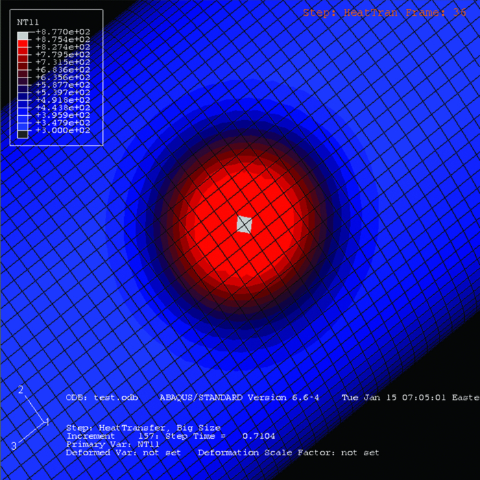
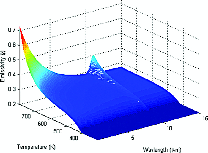
This relationship is plotted in Fig. 7 and illustrates the increasing nature of emissivity, and therefore an associated decrease in reflectance, as a function of temperature with a corresponding decrease as a function of wavelength. This decrease in reflectance as a function of temperature is particularly strong in the shortwave infrared and strongly affects the results of the current study. Also note the inclusion of the strong oxidation peak at ∼10.5 to 11 μm.

Fig. 7

Wavelength and temperature dependent emissivity for bare aluminum.

Prior to application of the BRDF model, the test object is projected onto the remote observer's line of sight, which varies as a function of time in the current study, thus establishing the correct geometry. The observer can either be in the plane of the incident laser, or out of plane.

2.D.

Sensor Model

The sensor model of the Remote Observer Scenario Toolkit includes a wide range of effects. Image blur due to the effects of diffraction, jitter, turbulence, drift, detector size, and wavefront error are applied as optical transfer functions (OTFs).^{2, 3} Figure 8 contains 3 bar chart test results of the OTFs across 5 wavelength bands from the shortwave (1.315 μm) to longwave infrared (10 μm). In this example the shortwave infrared wavelength results are dominated by turbulence and detector size, while at the longer wavelengths diffraction effects dominate.

Fig. 8

Three bar chart blur test results for the 5 sensor bands, reflected in-band (1.315 μm) in upper left, MWIR 1 (3.9 μm) upper center, MWIR 2 (4.7 μm) upper right, LWIR 1 (8.0 μm) lower left, LWIR 2 (10 μm) lower right. At the shortwave infrared wavelength results are dominated by turbulence and detector size, while at the longer wavelengths diffraction effects dominate.

Any spectral waveband can be built via application of spectral response functions to input high spectral resolution data. Sampling effects arising from any focal plane design can be represented to include spatial offset between bands. Radiance-at-the-sensor aperture images are radiometrically converted to irradiance at the focal plane, which is in turn converted to photoelectron images. Analog-to-digital conversion, well depth limits, and noise processes effects can also be applied.

3.

Results

The test object evaluated in the current study is a faceted aluminum cylinder with facets 5 mm × 5 mm in size. All facets are of the same area, and are defined by the facets setup in ABAQUS. The facets are treated as planes with defined normal vectors and locations.

The incident irradiance pattern, computed using SHaRE, is projected onto the test object. Temperature images as a function of time, based on the same SHaRE-generated irradiance patterns, taking into account a time varying coupling coefficient derived from the BRDF model, are developed in ABAQUS for the test conditions. These temperature data points, in conjunction with temperature dependent emissivity data derived from the BRDF model, are converted into midwave infrared (MWIR) and LWIR spectral radiance images. The wavelength and temperature dependent BRDF is applied to determine in-band reflectance in the direction of interest.

The inband-reflected radiance and emitted radiance spots are projected into the observer line of sight and appropriate atmospheric path effects are added to the radiance images. The placement of the observer can be any position relative to the test object. Path transmittance and path radiance effects are applied to create radiance-at-the-sensor-aperture images.

Figure 9 and the associated video depict the high spatial resolution truth data for bare aluminum, with the observer viewing the target with a look angle of approximately 45 deg which creates the elongated shape of the spots. Reflected in-band is on the left and corresponding temperature map generated with ABAQUS is on the right. Note the reduction in reflected in-band radiance in the center of the spot at the point in time illustrated in Fig. 9 due to the temperature-dependent BRDF (i.e., coupling coefficient), consistent with the surface for bare aluminum in Fig. 7. Emissivity is rapidly increasing in the NIR as temperature exceeds 700 K, resulting in a corresponding drop in reflectance.

Fig. 9

High spatial resolution (truth) images, reflected in-band radiance on the left, corresponding temperature map on the right. Associated video captures nondegraded spot morphology with time with high spatial resolution reflected in-band radiance on the left and corresponding temperature map on the right. (wmv, 337 KB).

Figure 10 illustrates output from the Remote Observer Scenario Toolkit in which all sensor effects have been applied, a prediction of generated photoelectron units in 5 sensor bands for a single point in time during a test versus a receding target. The only noise applied in this example is shot noise. The associated video shows the evolution of the 5 spectral band signatures over the first 5 s following laser initiation. The color scale is different for each band and varies with time. Band 1 is a narrow shortwave infrared band, in band with the laser. Bands 2 to 5 are the thermal (midwave infrared and longwave infrared) bands and are centered in this example at 3.9, 4.7, 8.0, and 10.0 μm referred to as MWIR1, MWIR2, LWIR1, and LWIR2, respectively.

Fig. 10

Photoelectron images for 5 bands, reflected in-band (1.315 μm) in upper left, MWIR 1 (3.9 μm) upper center, MWIR 2 (4.7 μm) upper right, LWIR 1 (8.0 μm) lower left, LWIR 2 (10 μm) lower right. Associated sensor video captures time- and wavelength-dependent spot morphology with degradations due to atmospheric transmission and path radiance effects over 5 s following laser initiation. (wmv, 343 KB).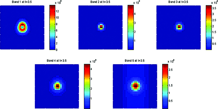

In this example, effects of wavelength dependent blur, wavelength and temperature dependent emissivity, and spatial sampling effects may be discerned. The effects of decreasing reflectance with temperature can clearly be seen in the video in the shortwave infrared band 1 as decreasing photoelectron count beginning at approximately t = 3 s. The four thermal bands share a common aperture and common pixel pitch. The increasing effects of diffraction with wavelength are evident in the thermal bands in Fig. 10, consistent with the blur test results of Fig. 8. At the beginning of the sequence the test object cylinder can be seen in the two MWIR bands primarily due to reflected sunlight. This weak reflected signal is quickly overwhelmed by the signature of the hot spot. The test object cylinder is evident much longer in the two LWIR bands due to the reflected signal of the warmer lower atmosphere and ocean surface, though toward the end of the sequence this signature is overwhelmed by that of the hot spot as well. In band 1 the reflected laser signal is vastly greater than the reflected solar energy from the test object cylinder.

Path radiance and path transmittance vary considerably across the MWIR and LWIR bands. Path radiance is much lower in the MWIR bands and LWIR2 exhibits the best path transmittance. For this airborne sensor example, once the laser is initiated the reflected laser and associated thermal signatures rapidly overwhelm path radiance contributions. Path transmittance effects differentially modify received signal strength across the spectral bands and must be taken into account when, for example, estimating pixel temperature.

4.

Summary

The AFIT/CDE Remote Observer Scenario Toolkit is a sophisticated, versatile, and unique model capable of simulating both dynamic, time-varying test object characteristics, and sensor performance for any combination of wavelength bands of any spectral width from the visible to the longwave infrared. An extremely wide range of worldwide atmospheric effects can be included and allowed to vary, line-by-line, across the spectrum. The model features true three-dimensional geometry on a round earth, and supports any relationship between the laser, test object, observer location, and solar position. The faceted target may have any orientation, and a spectrally and temperature dependent bidirectional reflectance distribution function, available for several materials, allows accurate calculation of reflected and emitted energy in any direction. The Remote Observer Scenario Toolkit is based on, and leverages, established community tools and legacy imaging model tools.

The Remote Observer Scenario Toolkit provides a high-fidelity, imaging simulation for the assessment and analysis of air or ground measurements of the results of laser tests. The simulation is data driven and can model any available camera system and all expected spectral effects. The atmospheric model, developed at AFIT, is the most complete model available within the community and accounts for fine scale effects in spectra due to aerosol and molecular absorption and scattering, and is most appropriate for laser effects simulations given its line-by-line nature. The imaging model includes degradations due to pixelization, blur, atmospheric, and noise effects. The kinematics of both the platform and the test object can be modeled in great detail.