3.1.

Field Data Collection

Field work was initiated in mid-December 2008 and completed in late January 2009 during the dry season. Leaves from red and black mangroves, representing various conditions, were collected from the top canopy branches with the aid of a hook. Regarding black mangroves, the conditions found included healthy tall black, dwarf black, and poor condition (i.e., degraded) black. Regarding red mangroves, only tall healthy and poor condition samples were located. For many of the tall healthy back and tall healthy red mangroves, the leaves were taken along the tidal channels from a boat using the hook apparatus. Specifically, the third through the fifth leaves from the tip of each branch were clipped so that only mature leaves were collected. In total, 90 samples of black mangrove and 60 samples of red mangrove were gathered, resulting in a sample size of 30 for each of the five stand types examined. All leaves were immediately placed in plastic bags and stored in a cooler at approximately 4°C prior to transportation to the laboratory for spectral reflectance analysis and pigment content determination.

3.2.

Spectral Response Measurements

An indoor black house laboratory was set up at the UNAM Instituto del Ciencias del Mar y Limnología Mazatlan Station in order to measure the leaf spectral responses. Canopy reflectance was measured using an ASD FieldSpec® 3 JR spectroradiometer (Analytical Spectral Devices, Inc., USA). The measurement range for this device is 350 to 2500 nm with a spectral resolution of 3 nm from 350 to 1000 nm and 30 nm from 1000 to 2500 nm. The sampling intervals of this equipment are around 1.4 and 2 nm for the visual/near-infrared and short wavelength/infrared regions, respectively. The output spectral data is resampled to 1 nm intervals, so there are, in total, 2150 bands for each spectral measurement. A 50 W halogen light was used as the light source for these indoor measurements. Each reflectance sample was measured based on two layers of mangrove leaves that were stacked facing upwards on a 25-cm diameter matt black plate. The sensor, with a 25-deg viewing angle, was mounted above the plate at a distance of 30 cm. A white reference (spectralon) was used every 5 min in order to calibrate the measurements. For each measurement, the number recorded was based on an average of 15 individual spectral measurements. Four of these average measurements were obtained for each sample by rotating the plate roughly 90 deg each time. These four measurements were then averaged for each sample. The spectral reflectance ($R$) was first converted to pseudo-absorption ($\log [1/R]$). The first and second derivatives were then calculated based on the difference in the pseudo-absorption values from two bands with a spectral distance of 2 nm and the range of wavelengths. The position of the red edge was determined using inverted Gaussian fitting using a nonlinear procedure,²⁹ which was followed by derivative analysis. Changes of the red edge position could be used to indicate vegetation conditions and quantify pigment content^21,30–32 because any decrease in chlorophyll content should decrease the absorption of red light. In addition, five vegetation indices—the Transformed Chlorophyll Absorption in Reflectance Index (TCARI),³³ the Gitelson and Merzylak’s Indexes (GMI),³¹ the Vogelmann’s Index (VOI),³⁰ the Carter’s Stress Index (CSI),⁷ and the Apan’s Water Index (AWI)³⁴—were calculated. These indices were selected to identify the spectral relationships of the pigments because they are known to be sensitive to vegetation conditions. TCARI was used to offset potential impacts of the nonphotosynthetic background materials.³² The CSI, GMI, and VOI all utilize the red edge wavebands that are sensitive to plant conditions.

3.3.

Leaf Pigment and Water Content Measurements

Following spectral measurements, a number of leaves from each sample were stored in paper bags for transport to a chemical lab where pigment and water content measurements were taken. Leaf pigment data were obtained using the pigment assay method provided by Zarco-Tejada.³⁵ A spectrophotometric analysis was then conducted to determine peak absorption at 646 and 663 nm. The leaf water content of the mangrove leaves was also determined using another portion of the leaf sample that was determined by the difference between the fresh and dry weight. The dry weight was calculated after the leaves had been oven-dried for 48 h at 60°C.

3.4.

Statistical Analysis

Analysis of variance (ANOVA) was used to examine the differences in spectral responses between the various mangrove species and their conditions. Specifically, responses were examined based on the mean reflectance at every 10 wavebands and the independent factors included the 215 wavelength regions (average reflectance of every 10-nm wavelength regions), the species, and their interactions. The same analysis was conducted by replacing the species with the mangrove condition. The Pearson’s correlation and linear regression were then utilized to examine the relationship between pigment content and spectral response. The coefficient of determination ($r^2$) was selected as the standard for determining the applicability of wavelengths and vegetation indices for the measurement of pigment content. These three statistical methods—ANOVA, Pearson’s correlation, and linear regression—were performed on the red mangrove sample (healthy and poor conditions), the black mangrove sample (healthy, dwarf, and poor conditions) and the entire sample (i.e., pooled). One healthy and two poor condition red mangrove individual samples were also excluded from the analyses because they were determined to be influential points (i.e., outliers that would have dramatically changed the regression equations). These three samples were considered abnormal samples that simply did not represent the conditions they were originally grouped into. To identify any potential influential points, an initial check was conducted using scatter plots. Using scatter plots, outliers can be easily recognized and, if far enough away from the mean, they can be identified as influential points. Four statistical measures (studentized residual, leverage, Cook’s D, and DFFITS) were then calculated to determine whether any outliers with extreme values should be removed for analysis. The conventional cut-off values of 3, $4/n$, $4/n$, and $2/\text{sqrt}(n)$ were used for the studentized residuals, leverage, Cook’s D and DFFITS statistics, respectively.

4.1.

Mangrove Pigment Content

As shown in Table 1, the species and condition of the mangrove significantly influence the pigment content. Regarding differences between the species, the red mangrove leaves show a slightly higher overall chlorophyll content ($\mathit{Chl}\mathrm{a}+\mathit{Chl}\mathrm{b}$) than the black mangrove leaves (47.8 versus $40.4\mathrm{mg}/{\mathrm{m}}^2$, $P<0.0001$). Moreover, the mean red mangrove Chl a level is also slightly higher than that of the black mangrove ($P=0.0012$). This discrepancy explains the differences between the species in regards to leaf color. Regarding condition, there are also significant differences in pigment content between healthy and poor condition mangroves. For the red mangrove, the Chl a and Chl b contents decreased by 17.9 and $5.5\mathrm{mg}/{\mathrm{m}}^2$, respectively ($P<0.001$ for both variables). Similarly, healthy and poor condition black mangroves showed significant differences in both Chl a and Chl b contents ($P<0.0001$). In addition, there were significantly lower Chl a ($6.2\mathrm{mg}/{\mathrm{m}}^2$, $P<0.0001$) and Chl b ($2.98\mathrm{mg}/{\mathrm{m}}^2$, $P<0.0001$) levels in poor condition black mangroves compared with dwarf black mangroves.

Table 1

Pigment content of mangroves based on species and condition (Mazatlan, Mexico).

Regarding the total carotenoid content, there was an observed mean decrease of $5.5\mathrm{mg}/{\mathrm{m}}^2$ ($P<0.0001$) in the poor condition red mangroves and a mean decrease of $2.1\mathrm{mg}/{\mathrm{m}}^2$ ($P<0.0001$) in poor condition black mangroves compared with respective healthy samples. The ratio of Chl a to the total carotenoid content, another indicator of changes in the total carotenoid content, also decreased from 1.8 to $1.4\mathrm{mg}/{\mathrm{m}}^2$ ($P<0.0001$) and 2.1 to $1.8\mathrm{mg}/{\mathrm{m}}^2$ ($P<0.0001$) for red and black poor condition mangroves, respectively.

Although the dwarf black mangrove leaf is often visually different from the healthy black mangrove leaf, the results suggest that they are not necessarily different in regard to pigment content. Relatively small differences in Chl a and Chl b contents were observed between healthy and dwarf black mangroves (Table 1). These differences were determined to be statistically insignificant ($P=0.130$ and 0.102, respectively). Regarding the total carotenoid content and Chl a/total carotenoid ratio, the $P$ values were significant at 0.039 and 0.024, respectively. In contrast, no significant difference was detected regarding the Chl a/total carotenoid ratio ($P=0.857$) between the dwarf and poor condition black mangrove. Consequently, the results suggest that it is more difficult to distinguish between the dwarf and poor condition black mangroves based simply on pigment content.

4.2.

Mangrove Spectral Properties and Leaf Water Content

Mangrove leaves display the typical vegetation curve, with high reflectance in the near-infrared (NIR) and low reflectance in the visible and short-wavelength infrared regions (SWIR) (Fig. 1). Reflectance in the visible region is lower than that in NIR due to chlorophyll absorption and leaf cell wall scattering. The lower reflectance in SWIR regions may reflect changes in the leaf water content. Similar to the pigment contents, there is considerable difference between the two mangrove species in regards to spectral reflectance, particularly in the NIR region. In contrast to healthy black mangrove, the red mangrove has a higher reflectance in NIR and SWIR and lower spectral reflectance in the visible region. The physiological condition also appears to influence the spectral response. In particular, poor condition mangrove has a lower reflectance in NIR and higher reflectance in the visible wavelengths and SWIR. The higher reflectance in the visible region explains the yellowish leaf color (i.e., chlorosis) of the degraded mangroves. The reflectance of NIR is principally controlled by the walls of the spongy mesophyll cells, with healthier leaves tending to have stronger reflectance in NIR as they reflect excessive amount of incoming energy in this region of the electromagnetic spectrum. In contrast, stressed leaves will have lower reflectance due to cell structure changes. The leaf water content is the main determinant of reflectance in the SWIR region. A higher leaf water content should theoretically increase absorption in SWIR and, thus, contribute to a decrease in reflectance. The higher reflectance of healthier mangroves in SWIR was unexpected given that one would assume that the healthier mangrove leaves should contain a higher water content. For the red mangroves, the water content actually increased from 64.7% in healthy leaves to 69.3% in poor condition leaves ($P<0.001$). Conversely, for black mangroves, both the dwarf (61.5%) and stressed black (62.0%) mangroves had lower water contents than healthy black mangroves (68.4%). The water content of stressed black mangroves was slightly higher than that of dwarf black mangroves, though no significant differences were observed ($P=0.536$). However, reflectance curves reported in a recent study²⁶ also showed decreased reflectance in the SWIR region for what are, presumably, degraded mangrove leaves. Consequently, this contradictory situation might signify other physiological factors, unique to mangrove leaves, which contribute to the spectral variation in this region of the electromagnetic spectrum. It is also worth noting that the spectral reflectance of the dwarf black mangrove is lower than that of the poor condition black mangrove in NIR and SWIR. This is contradictory to the higher reflectance in the visual light wavelength regions, where lower reflectance was observed for dwarf black mangrove. It has been reported that stressed mangroves shed leaves less often than healthy mangroves and stressed mangrove leaves are generally smaller and thicker.³⁶ These findings might explain the variations in SWIR and indicate that further work should be conducted to explore the impact of environmental degradation on mangrove leaf structure. In addition to all the differences, there are significant differences in the spectral responses measured in mangroves under various conditions ($P<0.0001$).

Fig. 1

Spectral curves of healthy mangroves (a), healthy and poor condition Rhizophora mangle (b), and healthy, dwarf, and poor condition Avicennia germinans (c) leaves. While reflectance in the visual light region is mainly influenced by leaf pigments, strong reflectivity in NIR can be caused by cell structure (cell wall scattering). Water content is the main influencer on shortwave infrared, and there are five main water absorption regions centered at 960, 1190, 1430, 1910, and 2700 nm (not shown).

4.3.

Relationship Between Spectral Response and Pigment Content

Although the water content in fresh leaves may decrease absorption in NIR and SWIR,³⁷ the results indicate significant relationships between pigment content and reflectance (or pseudo-absorptance) for a variety of wavebands. Two wavelength regions in particular, the green and the red edge, demonstrated strong to very strong correlations with Chl a and $\mathit{Chl}\mathrm{a}+\mathit{Chl}\mathrm{b}$ (Fig. 2). For Chl a, Chl b, carotenoids, and $\mathit{Chl}\mathrm{a}+\mathit{Chl}\mathrm{b}$, strong to very strong correlations were observed, mainly in the green light and red edge position, with the maximum correlation coefficients appearing around 560 nm and 705 nm, respectively. Because the main factor that influences spectral reflectance in the visible light portion of plant leaves is the pigment concentration^11,30 this result is what would be expected. In contrast, no strong correlations between reflectance in the red and blue light regions and pigment contents of the mangrove leaves were demonstrated. This would suggest that these wavebands are not sensitive to pigment content variation.¹¹ Regarding NIR and SWIR, only weak to moderate correlations were demonstrated. In general, the sum of Chl a and Chl b depicted extremely strong correlations with reflectance in the visible light region of all mangrove samples ($r=-0.83$, $P<0.001$). However, some correlation coefficients for chlorophylls at the species level (for red mangrove) were over $-0.9$ (data not shown). In contrast, correlations between total carotenoid content and spectral reflectance were weak to moderate.

Fig. 2

Correlogram of leaf Chl a content and pseudo-absorption of all mangrove samples. Two horizontal lines indicate the 0.05 significance level. The two thin line segments indicate strong absorption of Chl a and Chl b, whereas the thick line segment indicates the strong absorptive region for total carotenoids.

Applications of linear regression were used to examine the utility of selected wavebands for measuring pigment content because the data for the mangrove leaves (Fig. 3) were consistent with the general trend for linear relationships between chlorophyll content and spectral data. The results of the analyses (Table 2) suggest that spectral information from single bands around the red edge (690 to 750 nm) could be utilized to measure pigment content in these leaves. In particular, wavebands around 693 and 713 nm have a higher frequency of selection (Table 2) and, therefore, were selected as the most useful bands for pigment content determination. Models based on derivatives show relatively large coefficients of determination ($r^2$) (Table 2). In fact, the majority (77.7%) of the $r^2$ values depict values $>0.6$, which would indicate that hyperspectral remote sensing could be an efficient tool for pigment determination in these wetlands.

Fig. 3

Scatterplots of pigment versus derivatives (or vegetation index) for Avicennia germinans leaves. D, H, and P stand for dwarf, healthy, and poor condition, respectively.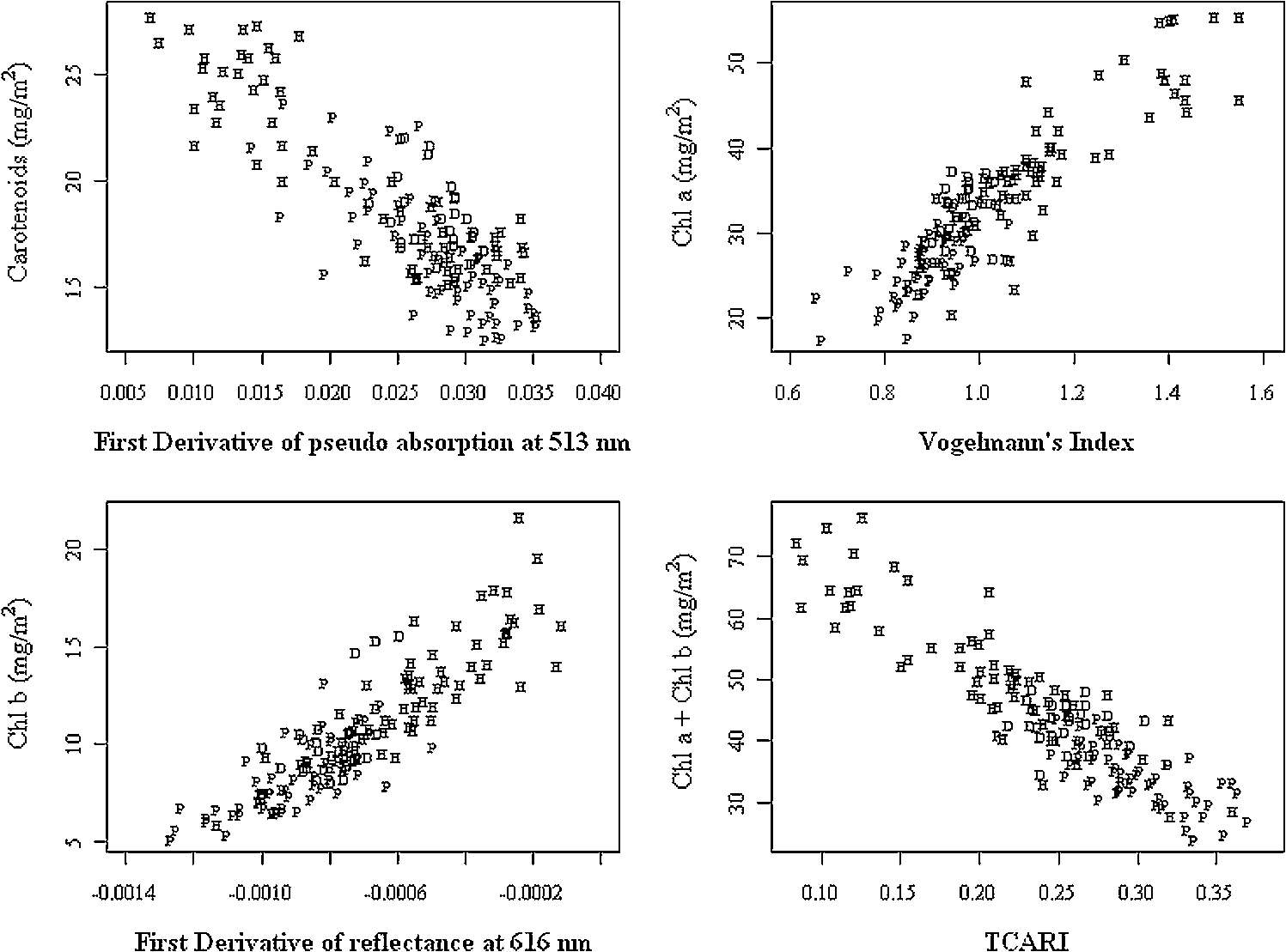

Table 2

Relationships between pigments and spectral data (black=A.germinans; red=R.mangle).

Table 3

Relationships between vegetation indices and pigment content (red=R.mangle; black=A.germinans).

Regarding species differences, most of the $r^2$ values for the black mangrove were lower than those of the red mangrove (e.g., Chl a and $\mathit{Chl}\mathrm{a}+\mathit{Chl}\mathrm{b}$). This result may be explained by the degree of degradation between the two species, with the poor condition black mangrove sample showing less degradation compared with poor condition red mangrove sample. Therefore, the larger contrast of the red mangrove would highly influence the linear relationships between the spectral responses and the chemical components. There are other wavebands within SWIR that are not listed in Table 2 that also show a high efficiency of prediction (e.g., 2032 nm for red mangrove, $r^2=0.611$). These relationships might be indirectly caused by nitrogen absorption because 2060 nm is a known nitrogen-absorption region.³⁸ In general, $r^2$ values for Chl b are lower than for those of Chl a, which may simply be the result of lower Chl b content within the leaves. In addition, many of the wavebands selected in Table 2 are in red wavelength region where absorption is dominated by Chl a.¹¹

In addition to the chlorophyll content, strong relationships were also demonstrated between the total carotenoid content and the spectral data, which was not expected given that previous studies have not reported such relationships.²¹ The results of this study (Table 2) indicate strong correlations for mangroves, particularly for the pooled (i.e., all) mangrove data. The waveband of 690 nm was negatively related to carotenoid content. Both wavebands 512 and 513 nm, which are unknown to be within the strongest absorption region of carotenoids, also showed strong correlations. This indicates that the wavelength region around 510 nm could be very useful for carotenoids determination in mangroves. Although the Chl a/carotenoid ratio has been reported as a good indicator of the carotenoid content,²¹ in this study this parameter was not found to be superior to the total carotenoid content for predicting carotenoid contents. However, the $r^2$ values for total carotenoid content and Chl a/carotenoid ratio were quite similar. The relatively large range of observed $r^2$ values (0.46 to 0.68) suggests the accurate mapping of the spatial distribution of the total carotenoid content in mangroves is possible with these data. However, it is recommended that more experiments be conducted to verify this claim.

4.4.

Vegetation Indices and Pigment Measurements

Previous studies have suggested that vegetation indices can be very useful for extracting pigment information.³⁹ However, in this investigation, these vegetation indices did not increase the ability of prediction. The $r^2$ values of many of the calculated vegetation indices (Table 3) were smaller than for those of single wavebands (Table 2). For example, the VOI demonstrated the highest potential for the prediction of Chl a with an $r^2$ value of 0.788, which is only 0.003 higher than that of waveband 694 nm. Only a few indices (e.g., TCARI) were able to slightly enhance the $r^2$ value (Table 3). TCARI is also the index that has the highest frequency for chlorophyll content prediction (Table 3).

4.5.

Red Edge Position and Pigment Content

Similar to others studies,²¹ the results of this study indicate roughly positive relationships between red edge positions and chlorophyll concentrations. Healthy red mangroves have longer red edge positions than those of tall healthy black mangroves (751 and 746 nm respectively, $P=0.001$). The red edge positions of the dwarf black and the tall black mangrove are relatively close (744 and 746 nm, respectively, $P=0.017$), which is expected since both are in healthy conditions. In contrast, the poor condition red mangroves’ red edge position was found to be around 740 nm. Fairly strong $r^2$ values were calculated for the red edge position and the Chl a content (Fig. 4). A linear regression model, fitted to examine the relationship of all mangrove samples, indicated a general trend of longer red edge wavelengths for healthy mangroves and shorter red edge positions for poor condition mangroves. The dwarf mangroves’ red edge positions were found between those of the healthy and the poor condition mangrove with some overlap between these two conditions. Consequently, the red edge position could be a good indicator of health. Four tall healthy black samples showed small red edge positions (739 to 742 nm). Interestingly, these samples also had lower than average water contents. The red edge position shift has also been shown to be related to water content and stress, with a slight loss in water content shifting the red edge to the longer wavelength region and with even more water loss, shifting it to the short wavelength regions.⁴⁰ Consequently, the water content may have influenced the red edge position of these samples.

Fig. 4

Scatter plot of Chl a and the red edge position.