|
|
1.Introduction and ObjectiveRemote sensing provides large amounts of data to the scientific community in terms of spatial, spectral, radiometric, and temporal resolutions1 that can be used in a vast range of applications in agriculture,2 climate change research,3 urban management,4 ecosystems monitoring,5 and thematic mapping,6 among others. It is a very interesting field for evaluating the quality of lossy compression techniques. Lossy data compression facilitates accessing, sharing, and transmitting huge spatial datasets in environments with limited storage or with limited bandwidth. JPEG2000 is one of the possible lossy compression algorithms, and is currently an ISO standard.7 However, lossy data compression procedures modify the original information,8 and therefore rigorous studies are needed to understand the effects and consequences of this manipulation. Some previous works have analyzed these alterations in remote sensing images in different fields and with varying objectives: spectral analysis,9 digital classification,10 texture analysis,11 stereoscopy,12 and multivariate regression,13 among others. The present work aims at studying the effect of JPEG2000 lossy compression by determining the differences between the spatial pattern domains in the original image and the compressed image, and more particularly, the impact on the geostatistical usage of remotely sensed imagery. Comparing the geostatistical properties of compressed images before and after compression is a different and novel approach, explored here instead of the usual comparison of the global parameter peak signal to noise ratio (PSNR).14 Exploring and describing the spatial variation in images is one of the main applications of geostatistics in remote sensing15 as it can provide parameters for describing spatial patterns,16 measurements for spatial autocorrelation,17 procedures for downscaling images,18 tools for estimating continuous variables,19 data for radiometric coregionalization analysis,20 and optimal sampling designs for ground surveys.21 The variogram is an appropriate tool often used in geostatistics to carry out exploratory analyses.22 Section 2.4 of the present work outlines this geostatistic tool and its specific characteristics when it is applied to remote sensing images. It is, however, a particularly slow procedure for processing large amounts of remotely sensed data. This computational constraint makes it necessary to use distributed environments, such as high performance computing (HPC). HPC provides methods and infrastructures for distributing computation in order to reduce the total execution time. Some examples of the benefits of HPC applied to remote sensing are hyperspectral image modeling,23 fire monitoring,24 meteorological applications,25 image processing,26 some classification methods27 and web grid environments,28 among others. In this work, parallel computing plays an important role in allowing us to perform spatial pattern analyses within an acceptable period of time. Section 2.5 details the architecture, design paradigm and language, and programming libraries, as well as results in time execution performance in order to generate variogram analyses in an efficient scientific environment. Many different cases were studied in order to obtain robust conclusions regarding the main questions raised: is the degradation similar at short and far distances applying different compression ratios? Do the analyzed compression methods modify patterns at different directions? Do possible pattern alterations depend on three or two dimension compression methods? Are the short and large remote imagery series behaviors similar in spectral and time dimension? The rapid generation of variograms allowed applying these massive analyses to:
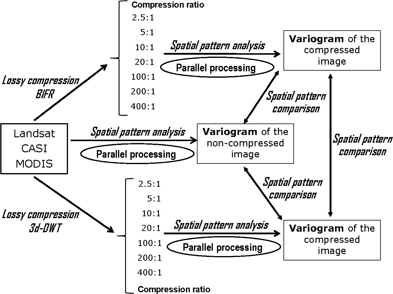
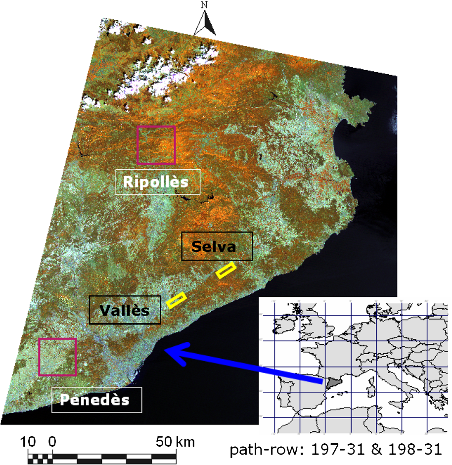
This complete test bed is detailed in Sec. 2.1. These different scenarios allow studying the possible spatial pattern alterations generated by the lossy compression methodologies and exploring the magnitudes and properties of these hypothetical changes. The conclusions of the work provide recommendations in each specific case about applying JPEG2000 lossy compression algorithms to remote sensing images for geostatistical analysis purposes. 2.MethodologyThe proposed methodology is a chain of image processing, lossy compression procedures, and geostatistical analyses in an HPC environment. Figure 1 shows the different stages and elements of this methodology as well as the position of the parallel task within the processing chain. These stages are detailed in the following subsections. 2.1.Materials2.1.1.LandsatIn this study, four scenes of multispectral (seven bands) Landsat-5 Thematic Mapper (TM) images have been used.29 The images selected for this work correspond to the dates 13-4-2006, 02-7-2006, 19-08-2006, and 11-9-2006, and cover two areas of about (spatial resolution of 20 m) of the 197-031 and the 198-31 path-rows. They thus provide a set of images that is very representative of the main phenological cycle in this Mediterranean region. These two areas, in the Ripollès and Penedès counties, (Fig. 2, pink squares) are located in Catalonia, a region of approximately situated in the northeast Iberian Peninsula at the extreme southwest of Europe (map location Fig. 2). The main landscape of the Ripollès region is deciduous forest, while the Penedès region has a vineyard landscape. Landsat images were chosen because they are the remote sensing images most used for research purposes in different applications,30 and they are also used in a large variety of applied projects.31 2.1.2.CASIThe compact airborne spectrographic imager (CASI) is an optic sensor for hyperspectral scanning based on a small CCD bar. In this study, two images (provided by the Institut Cartogràfic de Catalunya, ICC) with 72 spectral bands from red to near infrared (409.15 to 955.70 nm and an average bandwidth of 7.6 nm) were used. 32 The two scenes selected correspond to 18-05-2007 and 19-06-2007. For these two dates, two different study areas of at a spatial resolution of 3 m (Fig. 2, yellow rectangles) called Vallès and Selva located in the Montseny region, a mountain landscape in Catalonia. CASI images were chosen as an interesting test bed for three-dimensional compression methodologies (hyperspectral images are large radiometric third dimension examples). 2.1.3.MODISA moderate resolution imaging spectroradiometer (MODIS) Surface Reflectance Daily L2G Global 250 m product33 was used in this study as an example of a large time series dataset used for analyzing the geostatistical patterns of compressed and noncompressed images. The time series include 73 selected cloud free images from 2007 (from 5-5-2007 to 30-09-2007) from the same regions as the two Landsat images analyzed (Penedès and Ripollès), but covering a more extensive area. Higher spatial resolution MODIS bands were used, i.e., the near infrared and red spectral bands. The region covered is a square of centered in the square of the corresponding Landsat dataset. The study area of MODIS images was expanded in order to obtain a number of pixels with a resolution of 250 m large enough for statistical purposes, in this case . In summary, this remote sensing material was selected because Landsat images are used most widely, CASI serves to extend the third spectral dimension, and MODIS serves to extend the third time dimension tests. Both CASI and MODIS provide large datasets, which improves the lossy compression analyses. 2.2.Image ProcessingDifferent image processing methods were applied for each type of image depending essentially on the previous image processing level and on their particular characteristics. Landsat images were acquired at the L1G processing level, and were then georeferenced and radiometrically corrected with MiraMon GIS software34 according to the methodologies detailed in Refs. 35 and 36, and applied to the SatCat server.37 The optical reflectance range of the corrected images extends from 0 to 10,000, representing the % of reflectance*100, and so numbers were written with two decimal places in a short integer. This factor and type of data (signed short integer) are also used to represent the possible range of ground temperatures in °C (derived from the radiometric correction) of the TM thermal band. All images use a value to represent nodata regions, which in this case are normally caused by sensor problems or by post-processing artifacts. Defining the nodata value as is not arbitrary because nodata values that are defined too far from the valid data range can negatively affect normalization compression procedures.38 Consistent treatment of nodata values is one of the keys to performing correct image processing and subsequent data analysis. However, CASI images were acquired geometrically georeferenced using the SISA system developed by ICC.39 The flight orientation was SW-NE, which resulted in the geometrically corrected image being very large (), and therefore the CASI images were rotated with respect to the north projection in order to reduce the large amount of nodata pixels. The value range, data type and nodata definition in the CASI images were unified to match those of the Landsat images, also using the MiraMon software. Finally, the MODIS images were downloaded from the Warehouse Inventory Search Tool40 as a georeferenced reflectance product. It was only necessary to clip them to the study regions already detailed in the previous section and unify the nodata values. 2.3.Lossy CompressionThe reflectance product obtained was compressed at a wide range of different quality levels with the following compression ratios (CR): , , , , , , and (from soft to hard compression). Two methodologies, based on the JPEG2000 lossy compression procedures, were evaluated in this work:
Both compression procedures were applied using the Kakadu software,41 which is a complete implementation of the JPEG2000 standard, Part 1, completed with a great deal of Part 2 and 3.42 The BOÍ software,43 an implementation of the JPEG 2000 (Part 1) standard, was used for calculating the PSNR quality compression indicator in reference to noncompressed images. 2.4.GeostatisticsGeostatistics is a subset of statistics specialized in the analysis, interpretation, and inference of geographically referenced data.44 It was initially developed by Matheron45 and defined as a set of methods for studying the spatial distribution of a variable from a statistical approach in order to estimate the corresponding unknown value of a particular location or simulate its variability. When this variation has a spatial structure, the regionalized variable theory makes it possible to take spatial properties into account following a stochastic approach, and assumes a constant local mean and a stationary variance of the differences between regions separated by a given distance and direction.46 The variogram (also referred to as semivariogram) is based on these previous assumptions and, as defined in Eq. (1), it plots the variance function depending on sample distance separation and, consequently, the spatial patterns analyzed. This expression implies, for remote sensing images, that pixel values variance is only a function of distance and direction between pixels; then, there is no dependence on their particularly locations and, in statistics sense, this variance pattern is stationary for all study regions. Therefore, the variogram describes the pattern distribution of image spatial resolution, and it can identify a study region, a subscene of remote sensing image in this work. Equation 1: variogram definition. Note that the dependence is on distance () and on the squared difference of values (pixel values), and independent of particular positions ( and ).The sampled variogram can be modeled and fitted by a continuous function to identify structural parameters that characterize the spatial pattern for any quantitative variable distribution, including, of course, those of remotely sensed images, as carried out here in this study and in other previous studies47 (Fig. 3). These parameters are:
For each specific geostatistical application, the key role parameter depends upon the focus of a particular spatial pattern analysis. For example, range is the most suitable for autocorrelation analysis, nugget for determining stochastic noise and sill for variability’s measurements. The total sill was chosen as the main quality measure shown in Sec. 3 for analyzing alterations in the spatial patterns at studied compression ratios and with different methodologies. Different selected plots were used for three sensors for several dates, bands, and regions, which made it possible to determine the complete variogram structure by comparing the theoretical plot in Fig. 3 with the experimental plots in Sec. 3. 2.5.Parallel SolutionMost variogram analyses are used to explore the spatial patterns of irregularly distributed samples.48 Variogram analysis is usually a previous step to interpolation (kriging), which is a process with a high computational cost.49 Nevertheless, the variogram analysis of remotely sensed images has higher computing demands to those of irregularly distributed samples. Indeed, a large number of pixels are involved even in geographically small scenes with a high or medium spatial resolution, and therefore a very large number of pairs are necessary to obtain the variogram. Table 1 compares four examples of the amount of data involved and the time necessary for executions running on a single, normal PC (Intel(R) Xeon (R) 3.0 GHz and 1 GB of RAM). Table 1Comparison of processing time of variogram analyses between two irregularly distributed point measurements and remote sensing images. The sparse irregular distribution corresponds to a network of weather stations, and the dense, irregular, distribution to a GPS network of altimetry measurements, both detailed in Ref. 44; the remotely sensed image corresponds to two (Landsat and CASI) of the three examples used in this work.
In this work, a large number of spatial pattern analyses have been executed. All spectral bands (the number of bands for Landsat, CASI, and MODIS are 7, 72, and 2, respectively) on several scene dates (4, 2, and 73) and in two different study regions were analyzed. In addition, the images were compressed at several compression ratios (eight in all cases) and compared with noncompressed images. This implied 504 analyses for Landsat, 2592 for CASI, and 2628 for MODIS. Performing all these analyses would be a very time-consuming process; a single CASI analysis takes 57,727 s (see Table 1). Therefore, a distributed environment was the most suitable solution for a complete and efficient study. In order to reduce the execution time, the authors carried out a parallel implementation of the variogram analyses. The master/worker programming paradigm was used in which the master process schedules, distributes, and coordinates the tasks executed by the worker processes. The code was written in ANSI-C language, including MPI (message passing interface) as a message-passing library (version 1.2.7) that is used by the master process to communicate with the worker processes. Since MPI has become a standard de-facto message passing library,50 this solution () guarantees portability to different computer platforms. The distributed load design51 is not specifically defined and optimized for the characteristics of the images used in this work. However, it is a flexible design, tested with a wide range of image dimension that maintains a good balance and scalability suitable for other studies with a wide range of image dimensions and cluster properties. The scalability solution (adapting point samples analysis from Ref. 49 to remote sensing image analysis in the present work) can be achieved by defining a relatively small load unit: of two image rows of pixels. Each worker analyzes all possible combinations of nonrepeated pairs between two rows of the image and returns the partial variance and distance of the pairs involved to the master. The master distributes tasks (rows of data) to workers, accumulates partial results and manages input (remotely sensed image) and output (resulting variogram) tasks. 3.ResultsTwo types of results are presented in this section: geostatistical and computational. The geostatistical results are a set of variograms that compare images compressed at different ratios and noncompressed images for three image types (Landsat, CASI, and MODIS) focusing on the spectral or time dimension and possible anisotropy. The total sill parameters of the theoretical variogram are shown in different tables, while the experimental variograms are shown in plots. The computational results are focused on performance analyses of the parallel solution. The example shown in Sec. 3.2 corresponds to Landsat executions, but the performance results are very similar for all the image types analyzed. 3.1.Variogram AnalysisAs explained above, lossy compression mechanisms modify the original data information. Figure 4 illustrates the effects of compression ratios on quality visualization of the images. In this figure, the central image is a noncompressed CASI example, the top image sequence corresponds to three BIFR compressed images; from left to right, it is shown increasing compression ratios and decreasing quality. The bottom image sequence corresponds to the same sequence improved using 3d-DWT techniques. This composition summarizes most of the results presented in this section, and the following tables and figures quantify these effects in a geostatistical sense using the variogram spatial pattern analysis. Fig. 4The effects of compression on a CASI image fragment from the Selva region: noncompressed in the middle, upper sequence of BIFR compression ratios: , , and . The images in the bottom sequence were compressed at the same ratios but the 3d-DWT method was used. All of them correspond to a 4-5-3 band composite image.  3.1.1.LandsatThe first plot of Fig. 5 is a representative result of the alterations in the spatial pattern caused by the lossy compression (BIFR in this case) mechanisms. The main alteration to the spatial pattern due to lossy compression is the reduction in data variability at high compression ratios (more than ), although at lower CRs (from to ) the variograms have very similar shapes and structural parameters (nugget, range and sill). Table 2 is a summary of the behavior of the total sill, which is the most representative parameter in this study, for two dates and two regions for the BIFR method. Comparing the sill between compressed and noncompressed images represents a measurement of the loss of detail and variability caused by a compression method for all Landsat spectral bands. Table 3 shows the same information in relation to the 3d-DWT compression method. As seen in Fig. 6, there are only small differences between the two methods for Landsat images with the highest CR. Therefore, the following tables and figures corresponding to Landsat images only show the results for the BIFR method. The next cases (CASI and MODIS) demonstrate that 3d-DWT is a more useful method for image series that are larger than Landsat image series. Fig. 5Variogram results of the BIFR compression method on a Landsat image from the Ripollès region on 02-07-2006, a multispectral view.  Table 2Two examples (Ripollès region on 02-07-2006, and Penedès region on 11-9-2006) of the variation in the variogram parameter total sill at different compression ratios for the BIFR method.
Table 3Two examples (Ripollès region on 02-07-2006, and Penedès region on 11-9-2006) of the variation in the variogram parameter total sill at different compression ratios for the 3d-DWT method.
Fig. 6Landsat variogram comparison between BIFR and 3d-DWT compression in relation to the original pattern.  The sequenced plot in Fig. 5 shows that there are no significant differences in the variogram shape between bands, although there are differences in band range variances, and consequently in structural parameters depending on the region of the landscape. Table 4 and Fig. 7 reproduce the same variogram spatial pattern in a temporal sequence for an example of the near infrared (4-nIR) band. Table 4Time comparison of variogram results (total sill) for BIFR compression of Landsat images from the Penedès region on the 1-B and nIR bands.
Fig. 7Date comparison of variogram results for BIFR compression of Landsat images from the Penedès region on the near infrared (4-nIR) band. 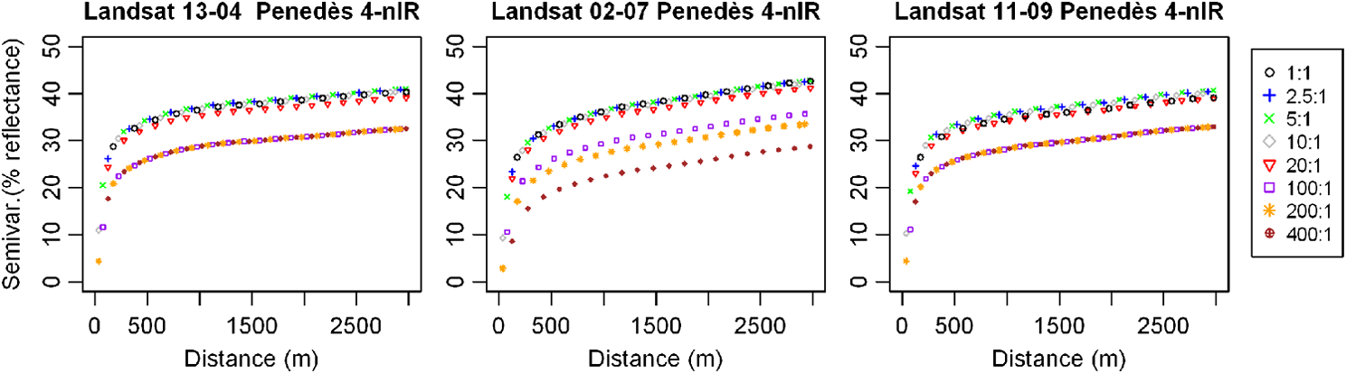 Furthermore, lossy compression may produce different variance alterations in relation to the spatial direction. In order to analyze this possible anisotropy modification, variance pattern at different azimuth angles has been studied. Figure 8 shows that the lossy compression mechanisms used in this work maintain the expected directional patterns at all compression ratios; thus, this result proves that the previous variograms were always omnidirectional. 3.1.2.CASIThe main characteristic of CASI images in relation to Landsat images is their higher spectral resolution (much more data in the spectral domain). The higher spatial and radiometric resolution are also notable, but they are not the focus of the present study. It is therefore an interesting test bed for exploiting three-dimensional compression methods. As it is impossible to show the results for 72 bands for two regions and two dates, the following figures display representative results for selected bands for different regions and dates. For example, Table 5 shows the total sill parameter of the 3d-DWT method for four selected bands (10, 21, 34, and 58) in the scene (19-06-2007), while Fig. 9 plots variograms at different compression ratios for three selected bands. Figures 10 and 11 show the variogram analyses of the scene for the two regions applying the 3d-DWT compression method. Table 5Total sill parameters for the k4p scene in the Selva region and for the complete sequence of compression ratios at four representative spectral bands.
Fig. 9Variogram results for the 3d-DWT compression method in the Selva region at selected CASI bands on 19-06-2007 ( scene).  Fig. 10Comparison of variogram results for the 3d-DWT compression method in the Selva region at selected CASI bands on 18-05-2007 ( scene).  Fig. 11Variogram results for the 3d-DWT compression method in the Vallès region at selected CASI bands. 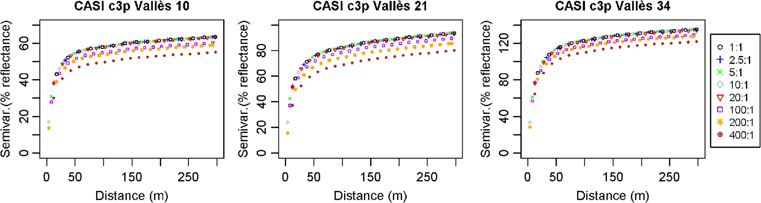 Table 6 shows the total sill parameter for the other scene ( on 18-05-2007) in the two study regions (Selva and Vallès) comparing the BIFR and 3d-DWT compression methods at selected CRs and bands (10, 21, 34). This table comparison demonstrates that spatial patterns have better fidelity with the 3d-DWT method than the BIFR method for CASI images. Figure 12 shows that 3d-DWT plots are closer to the noncompressed patterns, and that BIFR significantly alters the spatial patterns, especially for high compression ratios. Table 6Comparison between total sill parameters for the BIFR and 3d-DWT methods applied to the c3p scene in two regions at four representative compression ratios and three spectral bands.
3.1.3.MODISThe MODIS test bed allows a much larger amount of data to be explored in the time domain than the Landsat images because the MODIS daily revisit period makes it possible to obtain a large cloud-free time series. These series are especially appropriate for analyzing the pattern alterations of three-dimensional compression methods versus two-dimensional ones. The results for the MODIS images are similar to those obtained for CASI images, but both are different from the Landsat images. In these cases, the 3d-DWT method improves the quality of BIFR compressions. Table 7 shows that, at low compression ratios, 3d-DWT and BIFR maintain the spatial variability patterns of the original images, and that, at high compression ratios, BIFR loses quality compared to the 3d-DWT method. The plots in Figs. 13 and 14 (corresponding to the same region but to different spectral bands) show a reduction in the total sill parameter at increasing compression ratios for the 3d-DWT method, while Fig. 15 shows that 3d-DWT produces the pattern variability more faithfully than BIFR. Table 7Comparison between the BIFR and 3d-DWT methods of the total sill for four selected dates in the Penedès region for two spectral bands at representative compression ratios.
Fig. 13Comparison of experimental variograms of the 3d-DWT compression method for the Penedès region on three selected dates applied to MODIS images in the red band.  Fig. 14Variograms of the 3d-DWT compression method for the Penedès region on three selected dates for MODIS images in the near infrared band.  Fig. 15Comparison of variograms for the BIFR and 3d-DWT methods for three selected dates in the Penedès region at representative compression ratios for MODIS images in the near infrared band.  In summary, these results quantify spatial pattern alterations for lossy compression images depending on compression ratios, compression methods, and series dimension through analyzing differences between structural variogram parameters (focusing on total sill) of compressed and noncompressed images. These results shows that, for compression ratios higher than , the variogram is clearly degraded, reducing variability and thus, some capabilities or accuracy in related applications. This degradation could be partially solved, in some cases, by 3d-DWT, but this method needs a large amount of redundant data for significantly improve the BIFR method. These improvements are similar for time series and spectral series. This significant alteration (CR higher than ) could be relevant in several geostatistical studies of remote sensing images, such as geostatistical applications referred in Sec. 1 of this work, and for example, in landscape scale classification based on variogram analysis.52 In this example, if someone uses compressed remote sensing images instead of original images, and this compression is not done with the appropriate parameters, it could significantly alter classification results and, consequently, its main goal of determining the optimal support size (i.e., optimal spatial resolution) for characterizing forest ecosystems. 3.2.Performance ResultsAll the variogram analyses were processed using the IBM cluster of the research laboratory of the Computer Architecture and Operating Systems Department at the Universitat Autònoma de Barcelona. The IBM cluster is formed by 32 nodes, each with two Dual Core Intel(R) Xeon (R) 3.0 GHz processors with 12 Gbyte of RAM, and communicated with an integrated dual gigabit ethernet. Table 8 shows the average time of 14 independent executions using a different number of workers, while Fig. 16 shows the graphical representation and corresponding speedup evaluation.53 Table 8Execution time and speedup using n (0 to 24) workers.
Fig. 16Execution times (a) and speedup (b) with a different number of workers. The red dotted line corresponds to the theoretical linear speedup, while the blue line and points correspond to the empirical data. 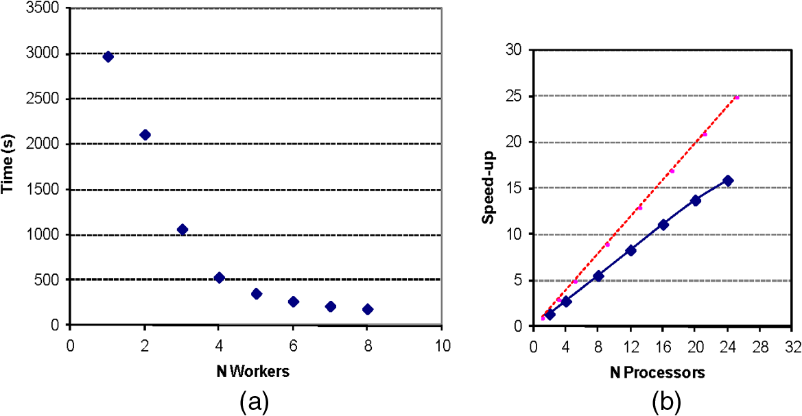 The proximity between the empirical speedup behavior and the theoretical linear speedup confirms that the parallel design and implementation provide a satisfactory solution for the computational problem at hand. These performance results demonstrate the validity of the proposed parallel solution, and the significant time reduction evidences the benefits of using distributed environments for processing large amounts of data, such as remotely sensed images. In fact, they provide an exhaustive test bed allowing running many executions with different parameters at several compression ratios in different regions on different dates, etc., and obtaining faster results and more agile comparisons. 4.ConclusionsThe main conclusions of this study on the alterations in the spatial pattern produced by JPEG2000 compression methodologies applied to remote sensing images are drawn hereafter:
Regarding to the computational methods developed in this work to reduce the execution time required for variogram analyses of remote sensing images: AcknowledgmentsThis work was partially supported by the Spanish government, by FEDER, and by the Catalan government, under Grants TIN2009-14426-C02-02, TIN2007-64974, PTA2010-3619-I, and SGR2009-1511. The authors are especially grateful to the Institut Cartogràfic de Catalunya, ICC, for providing the CASI data. Xavier Pons is a recipient of an ICREA Acadèmia Excellence in Research grant (2011 to 2015). Finally, the authors also wish to thank to the anonymous reviewers for their constructive comments that helped to improve the manuscript. ReferencesJ. R. Jensen, Introductory Digital Image Processing: A Remote Sensing Perspective, 3rd ed.Prentice Hall Series in Geographic Information Science(2005). Google Scholar
P. SerraX. Pons,
“Monitoring farmers decisions on Mediterranean irrigated crops using satellite image time series,”
Int. J. Rem. Sens., 29
(8), 2293
–2316
(2008). http://dx.doi.org/10.1080/01431160701408444 IJSEDK 0143-1161 Google Scholar
P. SchneiderS. J. Hook,
“Space observations of inland water bodies show rapid surface warming since 1985,”
Geophys. Res. Lett., 37
(22), L22405
(2010). http://dx.doi.org/10.1029/2010GL045059 GPRLAJ 0094-8276 Google Scholar
N. B. Changet al.,
“Change detection of land use and land cover in an urban region with SPOT-5 images and partial Lanczos extreme learning machine,”
J. Appl. Remote Sensing, 4
(1), 043551
(2010). http://dx.doi.org/10.1117/1.3518096 1931-3195 Google Scholar
K. Richteret al.,
“Plant growth monitoring and potential drought risk assessment by means of Earth observation data,”
Int. J. Rem. Sens., 29
(17), 4943
–4960
(2008). http://dx.doi.org/10.1080/01431160802036268 IJSEDK 0143-1161 Google Scholar
T. M. LillesandR. W. KieferJ. W. Chipman, Remote Sensing and Image Interpretation, 5th ed.John Wiley and Sons, New York
(2004). Google Scholar
D. S. TaubmanM. W. Marcellin, JPEG 2000: Image Compression Fundamentals, Standards, and Practice, 778 Kluwer Academic Publishers, Dordrecht
(2002). Google Scholar
T. RanchinL. Wald,
“The wavelet transform for the analysis of remotely sensed images,”
Int. J. Rem. Sens., 14
(3), 615
–619
(1993). http://dx.doi.org/10.1080/01431169308904362 IJSEDK 0143-1161 Google Scholar
G. Martínet al.,
“Impact of JPEG2000 compression on endmember extraction and unmixing of remotely sensed hyperspectral data,”
J. Appl. Rem. Sens., 4
(1), 041796
(2010). http://dx.doi.org/10.1117/1.3474975 1931-3195 Google Scholar
A. ZabalaX. Pons,
“Effects of lossy compression on remote sensing image classification of forest areas,”
Int. J. Appl. Earth Observat. Geoinf., 13
(1), 43
–51
(2011). http://dx.doi.org/10.1016/j.jag.2010.06.005 0303-2434 Google Scholar
M. A. Chaudhryet al.,
“Optimization of wavelet bases for texture analysis,”
in Proc. Fifth IEEE International Symposium on Signal Processing and Information Technology,
789
–793
(2005). Google Scholar
Y. Liet al.,
“Adaptive compression of remote sensing stereo image pairs,”
J. Appl. Rem. Sens., 4
(1), 041777
(2010). http://dx.doi.org/10.1117/1.3495716 1931-3195 Google Scholar
A. Zabalaet al.,
“Implications of JPEG2000 lossy compression on multiple regression modeling,”
Proc. SPIE, 6749 674918
(2007). http://dx.doi.org/10.1117/12.738028 PSISDG 0277-786X Google Scholar
M. KiefnerM. Hahn,
“Image compression versus matching accuracy,”
in International Archives of Photogrammetry and Remote Sensing,
316
–323
(2000). Google Scholar
P. J. CurranP. M. Atkinson,
“Geostatistics and remote sensing,”
Prog. Phys. Geogr., 22
(1), 61
–78
(1998). http://dx.doi.org/10.1177/030913339802200103 PPGEEC 0309-1333 Google Scholar
C. S. A. WallaceJ. M. WattsS. R. Yool,
“Characterizing the spatial structure of vegetation communities in the Mojave Desert using geostatistical techniques,”
Comput. Geosci., 26
(4), 397
–410
(2000). http://dx.doi.org/10.1016/S0098-3004(99)00120-X CGEODT 0098-3004 Google Scholar
R. G. Craig,
“Autocorrelation in Landsat data,”
in Proc. 13th International Symposium on Remote Sensing of Environment,
1517
–1524
(1979). Google Scholar
P. M. AtkinsonE. Pardo-IgúzquizaM. Chica-Olmo,
“Downscaling cokriging for super-resolution mapping of continua in remotely sensed images,”
IEEE Trans. Geosci. Rem. Sens., 46
(2), 573
–580
(2008). http://dx.doi.org/10.1109/TGRS.2007.909952 IGRSD2 0196-2892 Google Scholar
M. J. PringleM. SchmidtJ. S. Muir,
“Geostatistical interpolation of SLC-off Landsat ,”
ISPRS J. Photogram. Rem. Sens., 64
(6), 654
–664
(2009). http://dx.doi.org/10.1016/j.isprsjprs.2009.06.001 IRSEE9 0924-2716 Google Scholar
F. Chica-OlmoM. Abarca-Hernandez,
“Radiometric coregionalization of Landsat TM and SPOT HRV images,”
Int. J. Rem. Sens., 19
(5), 997
–1005
(1998). http://dx.doi.org/10.1080/014311698215838 IJSEDK 0143-1161 Google Scholar
M. A. OliverR. WebsterK. Slocum,
“Filtering SPOT imagery by kriging analysis,”
Int. J. Rem. Sens., 21
(4), 735
–752
(2000). http://dx.doi.org/10.1080/014311600210542 IJSEDK 0143-1161 Google Scholar
N. A. C. Cressie, Statistics for Spatial Data, John Wiley & Sons, New York
(1993). Google Scholar
A. J. PlazaC. I. Chang, High Performance Computing in Remote Sensing, Chapman & Hall/CRC Computer, Boca Raton
(2008). Google Scholar
A. Cortés,
“Half-duplex dynamic data driven application system for forest fire spread prediction,”
in Lecture Notes in Computer Science. High Performance Computing and Applications,
1
–7
(2010). Google Scholar
L. S. R. Froude,
“Storm tracking with remote data and distributed computing,”
Comput. Geosci., 34
(11), 1621
–1630
(2008). http://dx.doi.org/10.1016/j.cageo.2007.11.004 CGEODT 0098-3004 Google Scholar
J. Le MoigneW. J. CampbellR. F. Cromp,
“An automated parallel image registration technique based on the correlation of wavelet features,”
IEEE Trans. Geosci. Rem. Sens., 40
(8), 1849
–1864
(2002). http://dx.doi.org/10.1109/TGRS.2002.802501 IGRSD2 0196-2892 Google Scholar
M. K. Dhodhiet al.,
“D-ISODATA: a distributed algorithm for unsupervised classification of remotely sensed data on network of workstations,”
J. Parallel Distributed Comput., 59
(2), 280
–301
(1999). http://dx.doi.org/10.1006/jpdc.1999.1573 JPDCER 0743-7315 Google Scholar
S. Wanget al.,
“Simple grid toolkit: enabling geosciences gateways to cyberinfrastructure,”
Comput. Geosci., 35
(12), 2283
–2294
(2009). http://dx.doi.org/10.1016/j.cageo.2009.05.002 CGEODT 0098-3004 Google Scholar
National Aeronautics and Space Administration (NASA), Landsat Program http://landsat.gsfc.nasa.gov Google Scholar
A. C. Newtonet al.,
“Remote sensing and the future of landscape ecology,”
Prog. Phys. Geogr., 33
(4), 528
–546
(2009). http://dx.doi.org/10.1177/0309133309346882 PPGEEC 0309-1333 Google Scholar
X. Ponset al.,
“Ten years of local water resource management: integrating satellite remote sensing and geographical information systems,”
Eur. J. Rem. Sens., 45
(1), 317
–332
(2012). http://dx.doi.org/10.5721/EuJRS20124528 Google Scholar
L. Martínezet al.,
“Atmospheric correction algorithm applied to CASI multi-height hyperspectral imagery,”
in Proc. RAQRS II Valencia,
170
–173
(2006). Google Scholar
R. E. WolfeD. P. RoyE. Vermote,
“MODIS land data storage, gridding, and compositing methodology: level 2 grid,”
IEEE Trans. Geosci. Rem. Sens., 36
(4), 1324
–1338
(1998). http://dx.doi.org/10.1109/36.701082 IGRSD2 0196-2892 Google Scholar
X. Pons,
“MiraMon. Geographical information system and remote sensing software,”
(2013) http://www.creaf.uab.cat/MiraMon Google Scholar
V. PalàX. Pons,
“Incorporation of relief into geometric corrections based on polynomials,”
Photogram. Eng. Rem. Sens., 61
(7), 935
–944
(1995). Google Scholar
X. PonsL. Solé-Sugrañes,
“A simple radiometric correction model to improve automatic mapping of vegetation from multispectral satellite data,”
Rem. Sens. Environ., 48
(2), 191
–204
(1994). http://dx.doi.org/10.1016/0034-4257(94)90141-4 RSEEA7 0034-4257 Google Scholar
A. Zabalaet al.,
“JPEG2000 encoding of images with NODATA regions for remote sensing applications,”
J. Appl. Rem. Sens., 4
(1), 041793
(2010). http://dx.doi.org/10.1117/1.3474978 Google Scholar
R. AlamúsJ. TalayaI. Colomina,
“The SISA/0: ICC experiences in airborne sensor integration,”
in Joint Workshop of ISPRS WG I/1, I/3 and IV/4,
(1999). Google Scholar
Warehouse Inventory Search Tool, National Aeronautics and Space Administration (NASA),
(2011) https://wist.echo.nasa.gov/wist-bin/api/ims.cgi?mode=MAINSRCH&JS=1 Google Scholar
Geneva, Switzerland
(2004). Google Scholar
F. Aulí-Llinàset al.,
“J2K: introducing a novel JPEG 2000 coder,”
Proc. SPIE, 5960 1763
–1773
(2005). http://dx.doi.org/10.1117/12.633226 PSISDG 0277-786X Google Scholar
P. Goovaerts, Geostatistics for Natural Resources Evaluation, Oxford University Press, New York
(1997). Google Scholar
G. Matheron, Traité de Géostatistique Appliquée, Editions Technip, Paris
(1962). Google Scholar
M. A. OliverR. Webster,
“Kriging: a method of interpolation for geographical information systems,”
Int. J. Geograph. Inf. Sci., 4
(3), 313
–332
(1990). http://dx.doi.org/10.1080/02693799008941549 1365-8816 Google Scholar
C. E. WoodcockA. H. StrahlerD. L. B. Jupp,
“The use of variograms in remote sensing: I. Scene models and simulated images,”
Rem. Sens. Environ., 25
(3), 323
–348
(1988). http://dx.doi.org/10.1016/0034-4257(88)90108-3 RSEEA7 0034-4257 Google Scholar
C. D. Lloyd, Local Models for Spatial Analysis, CRC Press, Boca Raton
(2007). Google Scholar
L. PesquerA. CortésX. Pons,
“Parallel ordinary kriging interpolation incorporating automatic variogram fitting,”
Comput. Geosci., 37
(4), 464
–473
(2011). http://dx.doi.org/10.1016/j.cageo.2010.10.010 CGEODT 0098-3004 Google Scholar
“Introduction to MPI,”
Int. J. Supercomput. Appl. High Perform. Comput., 8
(3–4), 169
–173
(1994). http://dx.doi.org/10.1177/109434209400800302 IJSCFG 0890-2720 Google Scholar
I. Foster, Designing and Building Parallel Programs. Concepts and Tools for Parallel Software Engineering, Addison-Wesley(1995). Google Scholar
P. TreitzP. Howarth,
“High spatial resolution remote sensing data for forest ecosystem classification: an examination of spatial scale,”
Rem. Sens. Environ., 72
(3), 268
–289
(2000). http://dx.doi.org/10.1016/S0034-4257(99)00098-X RSEEA7 0034-4257 Google Scholar
M. CasasR. BadiaJ. Labarta,
“Automatic analysis of speedup of MPI applications,”
in Proc. of the 22nd ACM International Conf. on Supercomputing,
349
–358
(2008). Google Scholar
Biography Lluís Pesquer received his BS degree in physics in 1994 at the Universitat de Barcelona (UB) and a MS degree in computational science in 2009 at the Universitat Autònoma de Barcelona (UAB). He is researcher at CREAF since 2000 and he is currently the main developer of analysis tools, remote sensing modules and geodesy libraries of MiraMon GIS software. His main research interests are: spatial analysis, geostatistics, parallel computing in geoprocessing environments, remote sensing and applied geodesy to GIS.  Xavier Pons received his BS degree in biology in 1988, a MS degree in botany in 1990, a MS degree in geography in 1995, and a PhD degree in remote sensing and GIS in 1992, all from the Universitat Autònoma de Barcelona (UAB). His main work has been done in radiometric and geometric corrections of satellite imagery, in cartography of ecological and forest parameters from airborne sensors, in studies of the spectral response of Mediterranean vegetation and in GIS development, both in terms of data structure and organization and in terms of software writing. He has recently worked in descriptive climatology models, in modeling forest fire hazards and in analysis of landscape changes from long series of satellite images. He is Full professor at the Department of Geography of the Autonomous University of Barcelona and coordinates research activities in GIS and Remote Sensing.  Ana Cortés received both her first degree and her PhD in computer science from the Universitat Autònoma de Barcelona (UAB), Spain, in 1990 and 2000, respectively. She is currently associate professor of the Computer Architecture and Operating Systems Department at UAB. Her areas of interest are high performance computing, distributed and grid computing and also scheduling and load balancing in parallel systems. Her current research interest is focused on high performance computing applied to dynamic data driven applications systems for forest fire spread prediction.  Ivette Serral received her degrees in environmental sciences, MSc in remote sensing and GIS, both at the Universitat Autònoma de Barcelona (UAB), she is researcher at CREAF since 2005. The main objective of her work is to develop and manage GIS for the public administration: the Catalan marine and coastal information system, the Catalan healthcare information system, the Andorran environmental information system, etc. She developed new methodological tools in reference systems integration and multicriteria studies and Web geodata portals. She has been collaborating with secondary schools to disseminate GIS science and applications. |
||||||||||||||||||||||||||||||||||||||||||||||||||||||||||||||||||||||||||||||||||||||||||||||||||||||||||||||||||||||||||||||||||||||||||||||||||||||||||||||||||||||||||||||||||||||||||||||||||||||||||||||||||||||||||||||||||||||||||||||||||||||||||||||||||||||||||||||||||||||||||||||||||||||||||||||||||||||||||||||||||||||||||||||||||||||||||||||||||||||||||||||||||||||||||||||||||||||||||||||||||||||||||||||||||||||||||||||||||||||||||||||||||||||||||||||||||||||||||||||||||||||||||||||||||||||||||||||||||||||||||||||||||||||||||||||||||||||||||||||||||||||||||||||||||||||||||||||||||||||||||||||||||||||||||||||||||||||