

|
|
1.IntroductionWith global predictions of continuing mass coral bleaching events, increasing calls for government monitoring of reef environments and the question of coral adaptability, vulnerability, and change,1,2 it is imperative that methods to map, monitor, and manage reef environments be developed. The extensive areas covered by coral reefs in Australia alone mean that routine field monitoring can be conducted on only a very small subset of reefs. The long-term monitoring program at the Australian Institute of Marine Science annually surveys only 48 of the 3000-odd reefs that make up the Great Barrier Reef (GBR), a coverage representing just 1.6% of the reefs. Reef Check surveys are also conducted globally,3 but they cannot provide continuous and synoptic reef benthos information. Remote sensing is the only practical way to increase this coverage. 1.1.Mapping Coral Reef Benthic FeaturesThe progression of remote sensing in reef environments has been to (1) discriminate broad habitats or geomorphic zones with the available high and moderate spatial resolution multispectral data;4–10 (2) to determine differences in spectral response between common coral reef benthic features in situ using field spectrometers;11–18 (3) to evaluate spectral mixing and unmixing;19–21 and (4) to investigate the potential of object-based mapping approaches in these highly heterogeneous environments.22 As the development of coral reef spectral libraries led to an increased understanding of the controlling factors of reflection and absorption of light in reef environments, we are now in a better position to use this information to address the critical question of reef health through spatial and temporal variations in spectral reflectance across a reef. Coral reefs can be classified into broad habitat, benthic features, or geomorphic classes on a per-object basis using both high () and moderate (5 to 100 m) spatial resolution image data.4 However, the considerable heterogeneity of reef environments also means that despite the high spatial resolution image data now available, attempting to map benthic features will generally present an -resolution problem (i.e., where the feature of interest is smaller than the spatial resolution of the sensor).23 Pixel-based image classification routines assume an H-resolution image (i.e., the target is larger than the spatial resolution), where pixels are dominated by one cover type. This challenge has been faced in many terrestrial and aquatic environments where the goal is to map a continuous biophysical property or a portion of it, rather than place each pixel in a discrete category. This led to the development of spectral indices and spectral unmixing approaches.24 1.2.Coral Reef Health MappingTo use remote sensing effectively as an environmental monitoring tool, it is necessary to first determine features that are able to be mapped and indicative of the health of the environment in question. Environmental indicators have been successfully established in a number of globally important ecosystems, such as tropical forests, rangelands, wetlands, and oceanic areas.25 According to Hughes and Connell,26 indicators of stress on a reef include abundances of key organisms, population structures, species composition, and physical and chemical variables (i.e., salinity, turbidity, or nutrients). They also stress the difficulty in determining baseline values for these parameters across spatial and temporal scales, suggesting that more long-term studies are required to assess patterns of change and stability over time. Theirs was one of the few long-term studies of reef dynamics (see also Refs. 27 and 28). Such studies provide significant detail in a highly localized area, but they lack the large area or regional synoptic view of change that may be extracted from a temporal sequence of remotely sensed data such as the Landsat Thematic Mapper or SPOT Multispectral series of sensors. Holden et al. and LeDrew et al.29–31 argue that a measure of reef health may be extracted from moderate spatial resolution multispectral satellite image data (e.g., SPOT) through the use of spatial statistics. They suggest that phase shifts (e.g., coral to algal domination) may be extracted from a time series of data based on changes in benthos heterogeneity. This assumes that within the processed images, there will be known areas of “no change” to be used as a baseline, and that changes in the spectral values of benthos (and hence spatial heterogeneity) are great enough to be detected in one spectral band (in this case, a SPOT green band). An example of a potentially rapid change in reef/coral health is the onset of coral bleaching events. Mass bleaching has been successfully documented using IKONOS high-resolution multispectral data in the southern GBR.32 Indeed, the use of potential bleaching hot spots with sea surface temperature data and degree heating week indices are effective indirect uses of remote sensing in determining or predicting coral reef health.33 These methods have a common thread in that they all point to detecting changes in coral reef benthos, which in turn indicates reef health or stress. Therefore, if changes in reef benthic features can be detected or predicted using remote sensing products, programs can be developed for ongoing, remote monitoring of these ecosystems. This is similar in concept to the Ecological Health Monitoring Program for Moreton Bay (in southeast Queensland, Australia) where seagrass distribution and depth range is used as an indicator of ecosystem health based on the response to water column turbidity.34 Several indicators of reef health, status, or conservation value are documented,26,35 but few of these are appropriately simple or directly observable from remotely sensed data. Reef growth or deterioration over time is of global interest,1,36,37 and the amount of live coral cover may be used as a simple indicator of coral reef ecosystem health. Therefore, we propose that if the amount of live coral cover could be assessed using a spectral index, similar to vegetative indices in terrestrial environments, then this could be an ecosystem health indicator. If the amount of live coral cover and more specifically, its change over time in any location, can be accurately mapped, then an effective and quantitative assessment may be provided for reef conditions. 1.3.Mapping and Monitoring Using Spectral IndicesSpectral indices (e.g., the Normalized Difference Vegetative Index, or NDVI) are among the most common data transformations for mapping vegetation’s structural or physiological attributes. Part of the strength of these indices is that they are simple and relatively easy to implement from multispectral and hyperspectral data sets. The spectral band selection for these indices has been based on knowledge of the radiative transfer interactions in leaves and vegetation canopies.38 However, the indices are not deterministic models, although they rely on measured absorption (red) and scattering (NIR) processes, which are strongly negatively and positively correlated (respectively) to the chemical and structural properties of the vegetation present. Significant recent works have established the operational domain and improvements to ensure that they function in sparse to dense canopies, and in areas with significant atmospheric contamination.39 Although radiative transfer-based models provide accurate means to quantify biophysical properties (e.g., LIBERTY),40 they require the collection of specific atmospheric properties and complex algorithms and software. Indices offer a less complex method for estimating biophysical properties and may have potential for widespread use in coral reef environments if the environmental conditions (e.g., depth and benthic feature types) to which they are sensitive are established. If derived and applied appropriately, remotely sensed indices can provide a more easily and widely applicable method for mapping and monitoring environmental parameters than deterministic models. This is because they (1) do not require the user to implement complex radiative transfer equations (e.g., canopy-leaf scale or hydrologic optical); (2) can be applied with entry-level image processing software; (3) can be developed for multispectral and easily available data sets; and (4) only require preprocessing to at-surface radiance or reflectance values. As user expertise, computer processing capabilities, and cost effectiveness have been highlighted as challenges for remote sensing in coral reef management,41 a spectral index for mapping live coral cover may be a viable option. Within known limits and when using calibration data, indices are also a valuable method for determining and monitoring change and can be more sensitive in detailing fine-scale changes than categorical per-pixel classifications. This is because an index may identify radiometric change via an increase or decrease in value before that change is large enough to create a categorical change. For example, index values could indicate a decrease in forest biomass, where a categorical classification may require the forest to change completely to a cleared area for change to be noted. Hence, it is critical to ensure that the limits, or ranges of environmental conditions in which remote sensing indices work, are clearly defined. An example where this process has been followed is the development of vegetation spectral indices. These have been developed in response to mapping vegetation attributes and addressing environmental and temporal limitations to remotely sensed spectral response such as atmospheric and soil variations.42 While the use of spectral indices is commonplace for mapping and monitoring many different environments (e.g., SeaWiFS color products and AVHRR/MODIS/TM vegetation indices), to date, comparative indices that are sensitive to live coral cover or any other form of submerged aquatic vegetation have not been rigorously tested in the scientific literature. 1.4.Potential for Spectral Indices in Coral Reef MappingSpectral indices provide a method for mapping continuous variables. In a coral reef environment, benthic features vary across the reef according to numerous environmental conditions, including hydrodynamics, light quality, predation, and human influences. Changes in benthic cover patterns may therefore reflect a change in any of these environmental conditions. An effective spectral index will exhibit a direct response to relatively small changes in coral cover, across a range from low to high cover levels. The index will be more sensitive to small changes than a categorical per-pixel classification, which only reveals information about the most spectrally dominant benthic feature type, and assumes a discontinuous spatial distribution of the parameter of interest. Spectral indices are also very simple to implement, requiring minimal computer capacity or user expertise. However, they are usually bound by a certain range of applications.43 The survey completed by Joyce et al.41 and more recently by Roelfsema and Phinn44 indicated that the majority of reef scientists and managers are processing multispectral data at a simple level. Implementation of a spectral index would thus be appropriate. In addition, a large fraction of world’s reefs are in developing countries, so a useful index should ideally be able to be used with commercially available, cost-effective data and applied with minimal technical infrastructure. Due to this required simplicity, an effective index is more likely to be widely used than the deterministic/radiative transfer approach (e.g., spectral unmixing) and approaches requiring significant field-based training (e.g., classification). Spectral band ratios derived from image data have been used previously in reef environments to map bottom cover.45,46 However, when based on SPOT and Landsat image data, they are restricted to clear, shallow waters, especially when utilizing the red channel. Dustan et al.46 used 20 TM images of Key Largo, Florida, to calculate visible ratios in a time series to look at changes in bottom albedo over 14 years that showed a trend consistent with patterns of coral to algal domination, but the results were not statistically significant. Minghelli-Roman et al.17 documented discrimination of 14 coral genera based on simple band ratios from field spectrometer data, but they did not assess the discrimination between coral and other benthic cover types or test the applicability with image data. Early work by Hochberg and Atkinson12 also considered the separation of coral, algae, and sand based on linear discriminant function analysis with field spectrometry data, and then applied this to airborne hyperspectral imagery, with promising results. Each of these studies has laid the foundation for the work developed herein, where we build on past results by including spectral mixtures and water column simulations. Analysis of an image-based index does not require end-member identification (as per spectral unmixing) or complex ancillary data (as per hydro-optical models). Indices will function in both - and -resolution images, allowing areas to be described on a continuous and quantifiable (albeit relative) scale. A useful coral cover index must be robust and function in a range of typical conditions, considering atmospheric attenuation, varying water depths, clarity, and air-sea interface conditions. This paper describes preliminary analysis leading to index development for live coral mapping through the use of a spectral reflectance library obtained in situ from various locations in the southern and northern Great Barrier Reef (GBR), Australia,47,48 and Hawaii.49 The objective was to develop and test an index of live coral cover from in situ spectral reflectance data, and in doing so, determine its domain of application (limitations due to water depth and optical properties). This provides the basis for an image-based live coral mapping method to be described and rigorously tested in a follow-up paper. 2.Data and Methods2.1.Spectral Reflectance Data CollectionBetween 1999 and 2002, four field trips to Heron, Lizard, Yonge, and Eagle Reefs in the GBR were used to collect a substantial spectral reflectance library of common coral reef benthic features. The equipment and methods used for spectral collection have been detailed elsewhere.48 Reflectance spectra obtained at Lizard, Yonge, and Eagle Reefs (northern GBR) were recorded with both the target and sensor above the water’s surface. The remaining measurements were obtained below the surface, with negligible distance between the sensor, target, and reference. To supplement these data, the spectral reflectance libraries that were collected on Pandora and Orpheus Reef in the northern GBR47 and Hawaii49 were included (Table 1). All measurements are considered as reflectance, with negligible water or atmospheric contribution. Table 1Spectral library samples used for modeling mixtures. 2.2.Spectral Reflectance Data PreprocessingAll spectral reflectance libraries were resampled to match the University of Queensland’s Analytical Spectral Devices (ASD) UV-VNIR spectrometer’s band centers ) and bandwidths (full width and half ) between 400 and 700 nm by using the spectral resampling function of ENVI (Exelis Visual Information Solutions, Boulder, Colorado) and assuming a Gaussian distribution for each bandpass function. All reflectance spectra were then viewed in spectral space using the n-dimensional visualizer in ENVI to determine where clusters of similar reflectance spectra occurred that could be used to represent their respective benthic features. It became evident that there were six distinctive clusters, which corresponded to “blue” coral, “brown” coral,19 brown algae, green algae, sediment, and rock. Average spectra were then calculated from the reflectance spectra constituting each cluster, neglecting any reflectance spectra lying outside the dominant clusters. This method was considered preferable to simply calculating the average spectra of a particular category, as it meant that “spectral outliers” (possibly due to instrument or environment noise) could be discarded, and the selected “endmembers” were representative of the majority of the input. For the purposes of developing a simple index, blue and brown corals were later combined to create the “live coral” category. The resultant representative signatures were considered comparable in form and magnitude to those published extensively in the literature (e.g., Refs. 13, 14, and 16). The index is intended to be used to map live coral cover, and in doing so, that which is not “live coral” may be any other benthic feature found on a reef (e.g., dead coral, algae, sediment, rock, or rubble). Once the reduced library of six representative reflectance spectra (endmembers) was compiled, a linear mixing sequence was constructed with interactive data language (IDL)50 using the following equation: where is the mixed reflectance signal in band , is the number of endmembers, is the endmember reflectance in band , and is the proportion of endmember ; whereThe resultant mixed reflectance spectra were linear combinations containing between one and six input endmembers. Input proportions of endmembers or reef benthic feature types varied from 0% to 100%, in 5% increments. The simulated mixtures of benthic feature types represent the spectral reflectance signal recorded by a sensor with no water coverage or atmospheric contamination. Linear mixing may be a simplification of reality, but initial studies in this field have shown positive results for benthos discrimination thus far without employing nonlinear techniques.19,20 2.3.Spectral Transformations and Live Coral Index DevelopmentThe library of synthesized mixed reflectance spectra were resampled to match the spectral dimensions of several imaging sensors that will eventually be used for evaluating the live coral index at Heron Reef, southern GBR, Australia. These data sets included IKONOS, Landsat (Enhanced Thematic Mapper Plus), and a CASI-2 image data set containing 19 and 30 bands of image data between 400 and 800 nm. Resampling significantly reduced file size and enabled further analyses with spectral dimensions to match that of the CASI-2 image data acquired over Heron Reef at 1-m spatial resolution, which will be presented in a follow-up paper. With the exception of the IKONOS and Landat resampled spectra, data were transformed to estimate their first and second derivatives. An exhaustive series of simple ratios (, where and may be any band combination in the spectral reflectance domain of the synthesized mixed reflectance spectra library) and normalized difference ratios were then applied to the resampled data only, for use in determining the ratio band combination that was most sensitive to variations in live coral cover. Ratios for all possible band combinations (in the non-infrared bands) were computed in this manner, resulting in 240 band combinations.51 Band ratios could not be calculated for the full resolution spectra due to the large number of possible combinations. Thus, the results for band ratios and normalized band ratios will be presented only for the resampled CASI-2, IKONOS, and Landsat spectra. The synthesized spectral library containing original bands and their transformations (derivatives and ratios) for each spectral mixture was then used to determine wavelength regions most sensitive to modeled increases and decreases in live blue, brown, and total coral cover. This was done by individually calculating the linear correlation coefficient (Pearson’s ) between coral cover values and reflectance in each waveband or derivative/simple ratio/normalized ratio. Each was then plotted as the dependent variable against the individual waveband to create a correlogram. The band transformation or transformations with the highest correlation coefficient were then selected as the most sensitive to changes in live coral cover. 2.4.Water Column Optical ModelingResearch into coral reef remote sensing since the late 1990s has resulted in numerous studies seeking to characterize the spectral reflectance profiles of common reef benthic features (e.g., coral, algae, sediment). Further testing has been conducted to determine (1) the capabilities of different simulated sensors in detecting differences between benthic features;13,19,47 (2) how field spectra may be used to train image classifiers;52 and (3) theoretical mixing and unmixing scenarios.19,20 These past studies utilized high-spectral-resolution field spectrometer data obtained in situ, with little or no intervening water column. However in reality, satellite and airborne remote sensing of a reef without the effects of water column attenuation is not achievable. Light is absorbed and scattered throughout the water column due to dissolved and suspended material and the water itself. This acts to obscure the signal received from the benthos, making the retrieval of information about feature properties difficult. To address the effects of water column attenuation on benthos spectral separability, image classifiers, mixing, unmixing, and spectral indices, each of the aforementioned research projects could be repeated under varying water quality conditions and depths. Alternatively, it is possible to simulate these conditions based on optical radiative-transfer models such as Hydrolight53 Yamano and Tamura54 use Hydrolight to determine the limits for coral bleaching detection based on simulating changes in water quality (chlorophyll ), solar zenith angle, and atmospheric visibility. Here, a similar approach is used with Hydrolight 4.1 to ascertain the environmental limitations to the coral cover index. The six “endmembers” identified earlier were used as a basis for the modeling. The parameters of depth and water column chlorophyll content were varied to reflect values that could be reasonably expected across the reef. The testing here helped assess how robust the selected wavelengths were with respect to variations in water quality (represented by varying chlorophyll concentrations) and depth. Chlorophyll values representative of reef water variability on the GBR were taken from Brodie et al.,55 who reported mean and standard deviation concentrations from several locations with latitudinal and cross-shelf differences. In the absence of depth profiles of chlorophyll concentration, the average-depth weighted water column chlorophyll concentrations were used. The lowest concentration () represented Outer Shelf waters from Lizard Island–Cooktown, while the highest concentration () represented inshore waters from Whitsunday Island–Pompey Reefs. These values were taken for input to Hydrolight to represent extreme scenarios of water quality for testing the soundness of the coral cover index. Hydrolight 4.1 allows the user to specify one of six different inherent optical property (IOP) models to describe the water body. The chlorophyll-based model for sea water optical properties was selected.56 This required user input of chlorophyll only, suggesting that colored dissolved organic matter (concentrations of humic and fulvic acids) and two concentrations of suspended scattering particles (concentrations of terrigenic and biogenic particles) co-vary with the specified chlorophyll concentration. This assumption of covariance is a model limitation in this environment, where resuspended calcium carbonate sediment could also play a role. While keeping all other parameters constant (Table 2), the Hydrolight model was run six times, with all possible combinations of water depth (1, 5, and 10 m) and water column chlorophyll (0.33 and ), with the resultant signatures representing subsurface irradiance reflectance (). Table 2Hydrolight parameters used as input for modeling of spectral signatures at depth with changes in water column chlorophyll. Location was selected as Heron Reef, GBR, Australia, as this information will be used later with image data over this area. Similarly, the date and time was set to be within the image acquisition timing. Water depth was selected to cover a range of depths found on Heron Reef. Chlorophyll values are based on research in this region by Brodie et al.55 Cloud cover and wind speed were set to zero for simplicity.
3.Results and Discussion3.1.Spectral Processing and Live-Coral Index DevelopmentThe library of synthesized linearly mixed spectra contained 53,130 samples, each of which consisted of linear mixtures in varying amounts of the six identified endmembers (Fig. 1). For the purpose of this work, it was assumed that endmembers were entirely representative of their respective benthic features. It was also recognized that the data set could not cover all of the variability possible in the spectral mixtures likely to be encountered on coral reefs. In addition, the analysis presented in this paper does not consider the effects of target geometry/structure, water column (both of which may produce nonlinear mixing), air-sea interface conditions, or atmospheric attenuation. The latter three effects will be the subjects of ongoing research. These simulations therefore represent a best-case scenario for live coral index development using in situ spectral reflectance data. A summary of the various spectral resolutions, transformations, and the wavelength at which spectral reflectance was most significantly related to variations in live coral cover is presented in Table 3. This table also details the wavelengths that are most sensitive to variations in all benthic features used in this analysis. The general trend shows that derivatives and band ratios were consistently more sensitive to variations in the endmember composition than nontransformed reflectance spectra. It is also apparent that the correlation coefficient decreases with decreasing spectral dimensions (number of bands and increasing bandwidth) and that the most significant results are seen for the relationship between spectral data (reflectance or transformed reflectance) and sediment or rock. This information will prove useful in the future for mapping benthic features other than live coral. However, as the objective of this paper was to develop a live coral index, the results presented in the following sections will focus on the relationships between percent of live coral cover, derivative analysis, and band ratios. Table 3Summary statistics for linear correlation (pearson’s r) between live coral and various spectral transformations (reflectance, first derivative, second derivative, band ratio, normalized difference band ratio) and resampled spectral resolutions (full resolution, 19 band CASI-2, 30 band CASI-2, IKONOS, Landsat TM). ‘r’ denotes the highest value of Pearson’s linear correlation coefficient; and ‘λ’ denotes the wavelength at which the strongest correlation (highest r) was achieved. Band ratios for IKONOS and Landsat 5 TM broadband sensors are denoted using B, G, and R for blue, green, and red bands, respectively.
It is difficult to definitively determine the controlling factors of benthic feature spectral signatures. One of the main controls is the biological or pigment composition of the target; however, this does not account for all variability in the observed reflectance or absorption signatures.57 Nevertheless, Hochberg19 presented the results of a “pigment model” that simulated a spectral signature of a “brown” coral, taking into account the absorption maxima of chlorophyll , chlorophyll , -carotene, diadinoxanthin, and peridinin. Their predicted signature was very similar to their measured spectra. This accounted for the absorption of light by primary photosynthetic pigments but discounted fluorescence, scattering, and transmission controls. Considering only the absorption controls, the two documented pigments that occur only in zooxanthellae (corals) and not in red, green, or brown fleshy algae are peridinin and dinoxanthin. These pigments have absorption maxima at 475 and 570 nm58 (peridinin) and 418, 442, and 470 nm (dinoxanthin) (see Ref. 57 for a summary). Brown corals have been shown to have a reflectance peak near 570 nm as part of the “triple peak” reflectance pattern, whereas blue corals strongly absorb in the 580-nm region.13 Coral reflectance spectra are not only a product of their absorption controls. Fluorescence has been noted for its potential contribution to coral spectral signatures and may arise either from zooxanthellae or ectodermal tissue in the coral skeleton.59–61 Dove et al.62 suggest that much of the color attributed to reef building corals is due to green fluorescent proteins (GFPs), some of which play a role in the fluorescence contribution to the signature, while others are responsible for absorbing light. In contrast, however, Hochberg et al.14 suggest that there is little evidence in their data to suggest that fluorescence affects the basic shape of a coral spectral profile, but that it may act to enhance certain features. The functions of fluorescent tissue in the skeleton are not completely understood, and due to the infancy of florescence research, it is possible that there are still other pigments that have not yet been described chemically or spectrally.60 In addition, while pigments may be described within coral tissue, skeleton, and zooxanthellae, it has also been shown that morphology of corals and their interaction with sensor-viewing and illumination geometries alter the magnitude of the spectral signal received by a sensor.63 This is due to internal shadowing and light scattering within a coral colony. Thus, it can be seen that the relationship between coral spectra, index descriptions, and the controlling factors of light interactions is not simple. 3.1.1.Derivative analysisUsing both full-resolution spectra and those resampled to CASI-2 19 band resolution, it is clear that first- and second-order derivatives have a consistently stronger (higher correlation coefficient) and statistically significant relationship with the proportion of live coral contributing to the mixed signature than untransformed reflectance data (Fig. 2). When the combination of blue and brown corals is considered, the most sensitive transformations to variations in composition were the second derivative at 644, 625, 529, and 564 nm (, , , and 0.71, respectively). Mumby et al.64 also document a high level of distinction between living and nonliving corals around 562 nm and suggest this may be due to a fluorescence peak around 575 nm in coral spectral reflectance curves, though Hochberg et al.14 do not support a finding of fluorescence in this region. However, they do concede that it may be possible for fluorescence to enhance the spectral features. Compared with the full-resolution spectral data, the resampled 19-band CASI-2 data does lose spectral form due to fewer bands, and this is transferred to the derivative curves, resulting in the loss of small variations in peaks, troughs, and inflexion points. However, as the image data to be analyzed in the follow-up paper to this study has only 19 bands, it was appropriate to analyze the simulated data with the same dimensions. Simulations conducted by Lubin et al.65 suggest that due to atmospheric and water column attenuation, the most useful portion of the spectrum is further reduced to 400 to 600 nm. This therefore excludes the use of the two highest correlations that were found with second-derivative wavelengths (i.e., 644, 625 nm). Fig. 2Correlogram detailing the linear correlation coefficient between percent of live coral and in situ spectral reflectance; first derivative; and second derivative at wavelengths corresponding to 19 band CASI-2 image data. 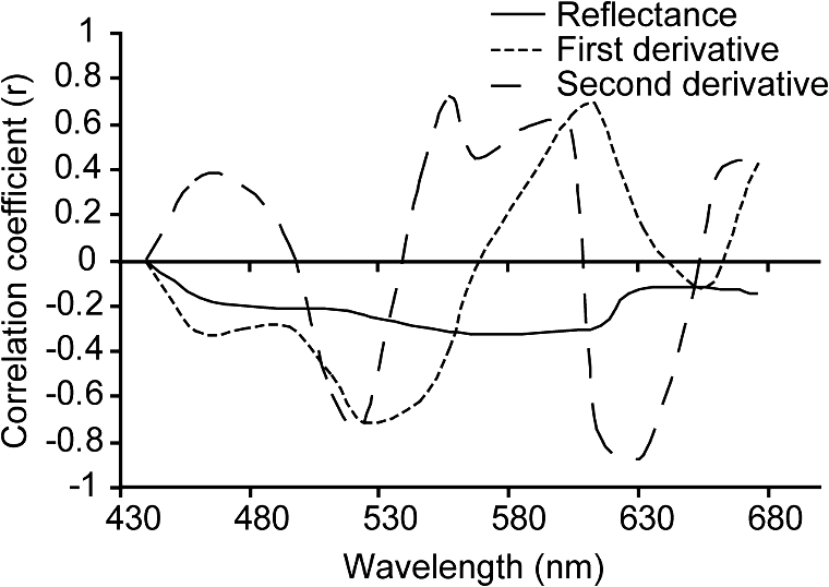 A complicating factor is that the correlation seen between coral composition and the band ratios and derivative bands is not only controlled by light-absorbing pigments characteristic of corals (i.e., coral skeleton, coral tissue, zooxanthellae), but by the gradual decreasing spectral contribution of the other cover types. Therefore, to develop a repeatable index, it is necessary to determine the biophysical controls on light absorption at these wavelengths and selectively choose ratios or derivatives that will consistently produce a result based on unique differences between corals and surrounding benthos. Hedley and Mumby57 provide a summary of the wavelengths of absorption maxima of pigments found in corals and algae, but as these overlap in some cases, it is difficult to definitively determine causal factors of spectral form. A detailed analysis of first- and second-derivative features of corals using the approach applied to sediments by Louchard et al.66 would provide the required information. As highlighted by Mumby et al.,64 it is very difficult to complete an exhaustive study on derivative analysis based on the number of different derivative orders that may be used and the start and end point of derivative calculation. Nevertheless, derivative analysis has been used quite frequently in the coral reef remote sensing literature for discriminating between common benthic feature types. Holden and LeDrew16 developed a decision tree using first-derivative analysis for detecting sand, macroalgae, and bleached and healthy coral. Despite conclusive evidence that coral spectral characteristics remain unchanged regardless of geographic location,13,14,16 the decision tree did not appear to be universally applicable.67 This technique was also applied only to pure endmember field spectra and did not incorporate the spectral mixing considered here. Fourth-derivative analysis has also been used in a similar fashion for identifying spectral features;12,18 however, this technique required highly smoothed spectral data that is not often obtained in a field environment.67 Many of the characteristic pigments found in corals exhibit absorption features in short wavelengths (; see Ref. 57 for a summary). The shorter wavelengths are less affected by water column absorption, but they also present a problem with both atmospheric and water column scattering.68 Water column attenuation is evident in all regions of the electromagnetic spectrum; the shorter wavelengths are more prone to scattering, while the longer wavelengths are affected more by absorption. Ideal band combinations will therefore lie somewhere between the extremes of scattering and absorption properties of atmosphere and water. 3.1.2.Band ratiosBand ratios produced similar results in terms of relationships to live coral cover, as did the analysis of derivative bands. A ratio of proved the most sensitive for estimating live coral cover composition () when using field spectral data resampled to CASI-2 19 band spectral resolution [Fig. 3(a)]. The CASI-2 sensor has a flexible bandset, and the band centers and bandwidths used for the image acquisition were selected to be useful for aquatic environments, so this analysis is somewhat biased in that the band ratios do not consider all the band centers of the full spectral resolution image data. However, as it was not possible to process the full-resolution field spectrometer data for all possible band ratios, analysis of the resampled 19 band data was considered appropriate. Fig. 3Linear correlation coefficients for the relationship between coral cover and all possible band ratio combinations for (a) spectra without water column influence; (b) simulated 1 m depth, chlorophyll; (c) simulated 1 m depth, chlorophyll; (d) simulated 5 m depth, chlorophyll; (e) simulated 5 m depth, chlorophyll; (f) simulated 10 m depth, chlorophyll; and (g) simulated 10 m depth, chlorophyll. Note that while the axes are evenly spaced, the bandwidths are not all equal; they are based on CASI-2 band positioning.  When using (resampled) broadband multispectral data such as IKONOS and Landsat TM, it can be seen that the highest correlation with live coral occurs within the blue and red bands. These are also the visible wavelengths most susceptible to scattering and absorption, respectively; thus, use of this broadband combination would be most effective on clear days with little atmospheric contaminants (, ) and in areas of shallow water (). Using these same bands, a variation of this ratio has been applied successfully for discriminating patch reefs from surrounding deeper lagoonal waters in Landsat data.6 The ratio was effective, as it significantly increased the contrast between deep water and patch reefs in the Heron Reef lagoon. A number of projects have used band ratios to map features in relatively shallow, clear-water environments. Mumby45 has successfully applied band ratios to quantify seagrass standing crop over sand. Seagrass chlorophyll content and light absorption by chlorophyll were used to justify the wavebands in the ratio. Chlorophyll content and (far) red light absorption were also found to be significantly related in coral, though this relationship could be used only for exposed or very shallow corals due to water column absorption at longer wavelengths.67 Predictably, this band ratio combination would also be affected by variations in water column chlorophyll when the benthos was submerged. Absorption of light by chlorophyll does not provide unique discrimination between corals and other benthos due to its presence in all photosynthesizing organisms (e.g., macroalgae, microalgae, seagrasses, clams, etc.). The scientific literature documents the wide degree of variability between coral spectral signatures. Past studies have shown that variations in measured spectral signatures will occur within a colony when measured at different locations on the colony,14 or from different viewing angles,63 though Minghelli-Roman et al.17 suggest that coral tissue pigment content influences the spectral signal more than coral morphology. However, it is also noted that differences at this scale are primarily seen in reflectance magnitude rather than spectral form. Band ratios and derivative indices are not affected by reflectance intensity variation, so long as the variation is consistent within the selected wavebands. 3.2.Water Column Optical ModelingTo test the effects of different water column properties on the index-based method for mapping live coral cover, changes in depth and water column chlorophyll were simulated. In the reflectance domain, addition of up to 10 m of water and chlorophyll made little change to the correlation coefficients observed for the relationship with live coral cover [Fig. 4(a)]. Regardless of the combination of depths and water column chlorophyll, the correlation coefficients per wavelength remained negative and low. The only exception to this pattern was seen at a depth of 10 m, where the chlorophyll content had a more noticeable effect at wavelengths greater than 600 nm. Fig. 4Linear correlation coefficients for the relationship between coral cover and (a) reflectance; (b) first derivative; and (c) second derivative using hydrolight 4.1 simulations of 1 m depth, chlorophyll; 1 m depth, chlorophyll; 5 m depth, chlorophyll; 5 m depth, chlorophyll; 10 m depth, chlorophyll; 10 m depth, chlorophyll. 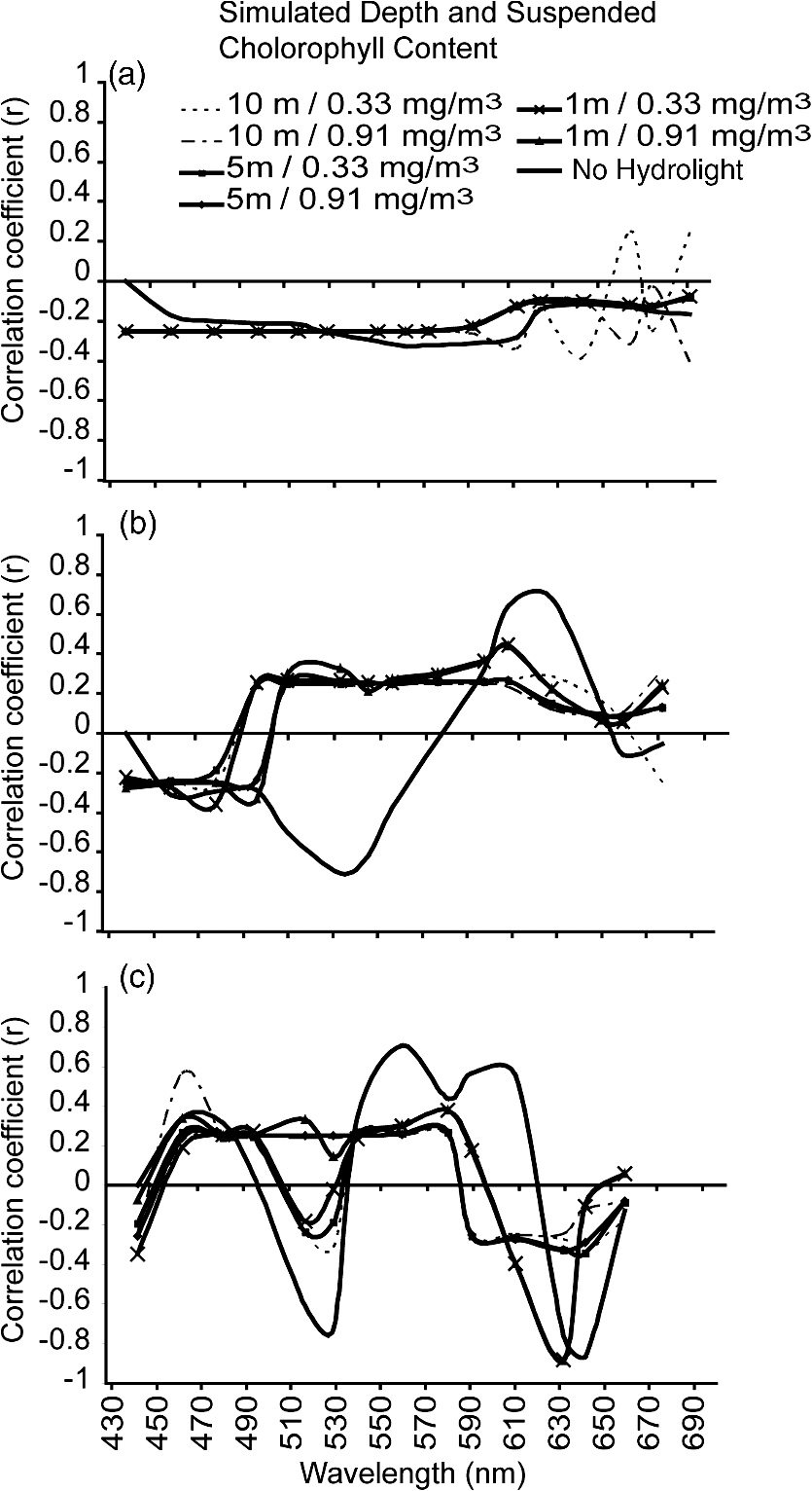 3.2.1.Derivative analysisWhen considering the relationship between first derivatives and live coral cover, it can be seen that simulating increased water depth and water column chlorophyll produced a noticeable effect in the wavelength region of 520 to 610 nm [Fig. 4(b)]. While the first-derivative spectra that had not been passed through the Hydrolight simulation predominantly exhibited a negative correlation with live coral cover in this region, all Hydrolight-simulated data followed different patterns. The correlation of live coral with the spectral derivative is considerably reduced by the addition of water. Addition of both depth (1 m) and chlorophyll () produced a change in correlation over all wavelengths; however, by increasing depth (5, 10 m) and chlorophyll () further, no further correlation change was observed. In summary, at a depth of 1 m with the lowest simulated chlorophyll (), the correlation between coral cover and the first derivative was the same as at a depth of 10 m and the highest chlorophyll (). Therefore, first-derivative analysis is relatively insensitive to water depth and quality variations once the feature is submerged. Analysis of the second-derivative correlations with live coral cover indicated that the correlations between reflectance/derivatives and coral cover decreased with the water column addition as shown in Fig. 4(c). However, some wavelengths were more affected than others. At wavelengths less than 490 nm, the addition of water and chlorophyll made little difference to the correlation curve. However, addition of the maximum chlorophyll changed the correlation coefficient to a positive value around 529 nm, regardless of the simulated depth. With either no water column or minimal chlorophyll addition, the correlation coefficient remained negative. The second derivative of 529 nm was previously identified as demonstrating a strong relationship with coral cover. However, due to the water column, chlorophyll-induced confusion, where the correlation coefficient changed from negative to positive, this wavelength was eliminated from the list of potentially useful data for mapping coral cover. The region around 564 nm was also identified as being sensitive to coral cover variations. After the Hydrolight simulations, the correlation with coral cover observed was weaker (lower correlation coefficient). After the initial addition of 1 m water depth and minimal chlorophyll, very little change was produced in the correlogram. This held true for the simulated maximum depths and water column chlorophyll. Selection of a wavelength or wavelengths that remained relatively insensitive to depth variations means that the index can be applied to an entire image without prior knowledge of water depth or quality. If a detailed and accurate bathymetric chart is available, it may be more appropriate and effective to first stratify the image and use the wavelengths most sensitive to coral cover at each depth. However, this would require considerably more processing time, and the increase in accuracy may not be significant. 3.2.2.Band ratiosThe effect of Hydrolight simulations on band ratios was also noticeable with band ratio correlations. The increase in water depth considerably reduced band ratio sensitivity at wavelengths less than 590 nm in the numerator, though curiously provided a region of increased correlation for numerators greater than 590 nm with denominators less than 516 nm. At 1 m depth, the increase in chlorophyll has little effect, with the pattern in band ratio correlations very similar between these two simulations [Fig. 3(b) and 3(c)]. At 5-m depths [Fig. 3(d) and 3(e)], the pattern is also very similar to that displayed for the 1-m simulations; however, the relationship with live coral cover is weaker (lower correlation coefficient). With the 10-m simulations for both values of chlorophyll [Fig. 3(f) and 3(g)], a similar pattern is evident, but the presence of regions of higher correlation coefficients ( and ) is apparent. This may suggest that the stronger relationship in these wavelength regions is an artifact of the water column addition; i.e., the chlorophyll increase over the 10-m water column is enough to change the signature sufficiently so that it is once again confused with coral at this depth. 3.3.Considerations for Development of an Image-Based IndexThe results presented in the preceding sections will be of use for regional and/or global mapping and monitoring of coral reef ecosystems only if the information can be translated to the scale of an airborne or satellite image pixel. This introduces several more challenges to be considered when scaling from field to image spectra. These challenges can be broadly defined as either environmental- or sensor-specific. 3.3.1.Environmental considerations for index developmentAtmospheric effects: Atmospheric attenuation is primarily prevalent in the scattering of shorter wavelengths. Lubin et al.65 and others suggest that atmospheric scattering (particularly at wavelengths shorter than 500 nm) produces additive path radiance effects that obscure many spectral features from satellite image data that are apparent in in situ field spectrometer data of reef substrates and benthic features. Nevertheless, several models are available for correcting images for these attenuating effects, and the derivative bands suggested here are not within the region of highly attenuated wavelengths. Variations in sea-state and distribution of sun glitter at the surface of the waterSun glitter results in reflection of large amounts of insolation at all wavelengths and obscures benthic features. This is particularly noticeable with high-resolution image data (e.g., nearly 50% of the IKONOS images received by Andréfouët et al.4 were significantly affected by surface sun glitter) and will saturate any index applied to affected data. Image-based correction is relatively simple and effective with both multispectral and hyperspectral data, provided that it contains a wavelength long enough to provide information on the sea surface only, rather than subsurface features, i.e., a near-infrared (NIR) wavelength that is absorbed at the water’s surface.48,69 Refraction at the air-sea interfaceAs with atmospheric effects, the effects of refraction at the air-sea interface can be accounted for during image processing using a top-down approach, where a calibration factor is used.70 From an image perspective, the refraction factor can be incorporated post atmospheric corrections and may be a considered a constant value, as any variations due to temperature and salinity are negligible.71 Failure to account for air-sea interface refraction should not affect the relative scale of the index, though it may produce errors in the absolute calibration. Variability of dissolved and suspended organic and inorganic matter in the water columnThe spatial variability in water column optical properties is a function of local and regional biological productivity and hydrodynamics.34 Optical properties may be affected by resuspension of sediments and circulation of nutrients due to tides, wind, and ocean swells. The effects of changing water column optical properties on index calculation have been addressed here in a simplistic manner through varying chlorophyll concentration in the Hydrolight model, though the spatial variability across a reef is unknown and assumptions of optical homogeneity are likely to be unfounded.72 Water depthSeveral image-based models are available in the literature for extracting bathymetric information from both hyperspectral and multispectral image data.66,73–76 The multispectral models tend to be relatively simple to implement and are based on the exponential decay of light with increasing water depths. The effects of water depth on band ratio and derivative correlations have been addressed to a degree within the scope of this project and led to the selection of a wavelength that is relatively robust for depth variations up to 10 m. Substrate topography and structureReef systems are inherently structurally complex and heterogeneous.77 Structural variability on reefs occurs across all scales of image pixels and will be particularly apparent with decreasing spatial resolution data. This means that individual pixels may contain not only benthic feature heterogeneity (corals, algae, sediment), but also different structures. This produces small-scale water depth variations and shadowing (e.g., within and between patch reefs/bommies) that have not been accounted for in the development of the index. These effects should not be too pronounced in high-spatial-resolution data (); however, the degree of variability in moderate spatial resolution data is a greater challenge. A useful and robust index must use wavebands that are least sensitive to variations in the above environmental effects. Alternatively, image data can be stratified accordingly using currently available simple models. However, the latter option is less favorable, as it involves additional processing routines, thus increasing the complexity of processing. This is contrary to the idea of a simple, easy-to-implement index. The extent to which each of the factors outlined above will affect the accuracy and effectiveness is not known, and it is suggested that further studies assess their contributions. 3.3.2.Sensor specific considerations for index developmentAll of the above environmental effects can vary both within and between image pixels. The degree to which the effects are observed will be a function of sensor spatial, spectral, and radiometric dimensions, in addition to viewing geometry. Within-pixel variations will be increasingly prominent with increasing pixel size, while between-pixel variations may be noticeable over all spatial dimensions. 4.Conclusions and Future ResearchBy using simulated linear mixtures of in situ field reflectance data to examine the relationship between live coral and spectral reflectance, second derivatives were shown to be the most sensitive to variations in live coral contributions to a mixed signal. While the second derivative at 644 nm returned the highest correlation (), this wavelength is more susceptible to absorption by the water column than shorter wavelengths. The second derivative at 529 nm () appeared a viable alternative with initial mixture and correlation testing; however, Hydrolight 4.1 simulations of up to 10 m water depth and additional water column chlorophyll suggested that second derivatives within this wavelength region were no longer suitable for submerged features. Therefore, the second derivative at 564 nm was considered a more suitable spectral band placed within a suitable window of visibility through the water column with minimal scattering and absorption of light due to water, dissolved organic matter, suspended organic matter, and suspended inorganic matter. Derivatives require a higher level of data processing than simple band ratios and were shown to be only marginally more sensitive to variations in live coral cover than individual bands and ratios. After testing all possible band combinations for simple band ratios, the combination of 594:625 nm was shown to be the most effective () when using data resampled to 19-band CASI-2 spectral dimensions. Decreasing spectral dimensions (decreasing number of bands and increasing bandwidth) resulted in decreasing sensitivity to live coral variations. The focus of this work has been on index development using in situ spectral reflectance data and simulated water column optical properties. This work will be followed by further quantitative testing and image analysis using hyperspectral CASI-2 image data of Heron Reef, in combination with detailed integration of field survey data for calibration and validation. The modeling results of this work have shown that the types of reef cover that are mixed within a pixel do affect the ability of different techniques to estimate live coral cover. For example, mixtures of sand with coral work well with our technique. Further work is required to identify in which mixtures can be resolved by empirical approaches, classification, and radiative transfer models. The final output of continuing study will be a fully refined live coral index that is tested for cost-effectiveness, accuracy, and ease of use with other currently available techniques for mapping reef environments. AcknowledgmentsThanks to Peter Scarth for assisting with computer programming, Chris Roelfsema for field assistance, and to Justin Marshall and Tiit Kutser/CSIRO Earth Observations Centre and Environmental Remote Sensing Group for the use of their spectral libraries and assistance with Hydrolight modeling. We appreciate the feedback from anonymous reviewers on an earlier version of this manuscript. ReferencesT. P. Hugheset al.,
“Climate change, human impacts, and the resilience of coral reefs,”
Science, 301
(5635), 929
–933
(2003). http://dx.doi.org/10.1126/science.1085046 SCIEAS 0036-8075 Google Scholar
O. Hoegh-Guldberg,
“Climate change, coral bleaching, and the future of the world’s coral reefs,”
Mar. Fresh. Res., 50 839
–866
(1999). http://dx.doi.org/10.1071/MF99078 Google Scholar
G. Hodgson,
“A global assessment of human effects on coral reefs,”
Mar. Poll. Bull., 38
(5), 345
–355
(1999). http://dx.doi.org/10.1016/S0025-326X(99)00002-8 MPNBAZ 0025-326X Google Scholar
S. Andréfouëtet al.,
“Multi-sites evaluation of IKONOS data for classification of tropical coral reef environments,”
Rem. Sens. Environ., 88
(1–2), 128
–143
(2003). http://dx.doi.org/10.1016/j.rse.2003.04.005 RSEEA7 0034-4257 Google Scholar
W. AhmadD. T. Neil,
“An evaluation of Landsat Thematic Mapper (TM) digital data for discriminating coral reef zonation: heron reef (GBR),”
Intl. J. Rem. Sens., 15
(13), 2583
–2597
(1994). http://dx.doi.org/10.1080/01431169408954268 IJSEDK 0143-1161 Google Scholar
K. E. Joyceet al.,
“Combining Landsat and Reef Check classifications for mapping coral reefs: a critical assessment from the southern Great Barrier Reef,”
Coral Reefs, 23
(1), 21
–25
(2004). http://dx.doi.org/10.1007/s00338-003-0357-7 CORFDL 1432-0975 Google Scholar
P. J. MumbyA. J. Edwards,
“Mapping marine environments with IKONOS imagery: enhanced spatial resolution can deliver greater thematic accuracy,”
Rem. Sens. Environ., 82
(2–3), 248
–257
(2002). http://dx.doi.org/10.1016/S0034-4257(02)00041-X RSEEA7 0034-4257 Google Scholar
D. L. B. Juppet al.,
“Remote Sensing for Planning and Managing the Great Barrier Reef of Australia,”
Photogram., 40
(1), 21
–42
(1985). http://dx.doi.org/10.1016/0031-8663(85)90043-2 Google Scholar
D. A. Kuchler,
“Remote sensing: what can it offer coral reef studies?,”
Oceanus, 29 90
–92
(1986). OCEAAK Google Scholar
S. Andréfouëtet al.,
“Typology of atoll rims in Tuamotu Archipelago (French Polynesia) at landscape scale using SPOT HRV images,”
Intl. J. Rem. Sens., 22 987
–1004
(2001). http://dx.doi.org/10.1080/014311601300074522 IJSEDK 0143-1161 Google Scholar
S. AndréfouëtC. Payri,
“Scaling-up carbon and carbonate metabolism of coral reefs using in-situ data and remote sensing,”
Coral Reefs, 19
(3), 259
–269
(2001). http://dx.doi.org/10.1007/s003380000117 CORFDL 1432-0975 Google Scholar
E. J. HochbergM. J. Atkinson,
“Spectral discrimination of coral reef benthic communities,”
Coral Reefs, 19
(2), 164
–171
(2000). http://dx.doi.org/10.1007/s003380000087 CORFDL 1432-0975 Google Scholar
E. J. HochbergM. J. AtkinsonS. Andréfouët,
“Spectral reflectance of coral reef bottom-types worldwide and implications for coral reef remote sensing,”
Rem. Sens. Environ., 85
(2), 159
–173
(2003). http://dx.doi.org/10.1016/S0034-4257(02)00201-8 RSEEA7 0034-4257 Google Scholar
E. J. Hochberget al.,
“Spectral reflectance of coral,”
Coral Reefs, 23
(1), 84
–95
(2004). http://dx.doi.org/10.1007/s00338-003-0350-1 CORFDL 1432-0975 Google Scholar
H. HoldenE. LeDrew,
“Spectral discrimination of healthy and non-healthy corals based on cluster analysis, principal components analysis, and derivative spectroscopy,”
Rem. Sens. Environ., 65 217
–225
(1998). http://dx.doi.org/10.1016/S0034-4257(98)00029-7 RSEEA7 0034-4257 Google Scholar
H. HoldenE. LeDrew,
“Hyperspectral identification of coral reef features,”
Intl. J. Rem. Sens., 20
(13), 2545
–2563
(1999). http://dx.doi.org/10.1080/014311699211921 IJSEDK 0143-1161 Google Scholar
A. Minghelli-Romanet al.,
“Discrimination of coral reflectance spectra in the Red Sea,”
Coral Reefs, 21
(3), 307
–314
(2002). http://dx.doi.org/10.1007/s00338-002-0249-2 CORFDL 1432-0975 Google Scholar
M. Wettleet al.,
“Fourth derivative analysis of Red Sea coral reflectance spectra,”
Intl. J. Rem. Sens, 24
(19), 3867
–3872
(2003). http://dx.doi.org/10.1080/0143116031000075945 IJSEDK 0143-1161 Google Scholar
E. J. HochbergM. J. Atkinson,
“Capabilities of remote sensors to classify coral, algae, and sand as pure and mixed spectra,”
Rem. Sens. Environ., 85 174
–189
(2003). http://dx.doi.org/10.1016/S0034-4257(02)00202-X RSEEA7 0034-4257 Google Scholar
J. D. Hedleyet al.,
“Spectral unmixing of coral reef benthos under ideal conditions,”
Coral Reefs, 23
(1), 60
–73
(2004). http://dx.doi.org/10.1007/s00338-003-0354-x CORFDL 1432-0975 Google Scholar
J. D. HedleyP. J. Mumby,
“A remote sensing method for resolving depth and subpixel composition of aquatic benthos,”
Limn. Ocean., 48
(1), 480
–488
(2003). http://dx.doi.org/10.4319/lo.2003.48.1_part_2.0480 LIOCAH 0024-3590 Google Scholar
S. R. PhinnC. M. RoelfsemaP. J. Mumby,
“Multi-scale, object-based image analysis for mapping geomorphic and ecological zones on coral reefs,”
Intl. J. Rem. Sens., 33
(12), 3768
–3797
(2012). http://dx.doi.org/10.1080/01431161.2011.633122 IJSEDK 0143-1161 Google Scholar
S. R. Phinnet al.,
“Mapping coral reef environments at high spatial resolution: the role of spatial statistics,”
in Intl. Symp. Rem. Sens. Environ.,
(2003). Google Scholar
T. M. LillesandR. W. KieferJ. W. Chipman, Remote Sensing and Image Interpretation, 6th ed.John Wiley & Sons, Inc., New York
(2008). Google Scholar
S. R. Phinnet al.,
“The role of integrated information acquisition and management in the analysis of coastal ecosystem change,”
Remote Sensing of Coastal Ecosystem Processes, Klewer Academic, Dordrecht, The Netherlands
(2006). Google Scholar
T. P. HughesJ. H. Connell,
“Multiple stressors on coral reefs: a long-term perspective,”
Limn. Ocean., 44
(3), 932
–941
(1999). http://dx.doi.org/10.4319/lo.1999.44.3_part_2.0932 LIOCAH 0024-3590 Google Scholar
J. H. Connell,
“Disturbance and recovery of coral assemblages,”
Coral Reefs, 16 S101
–S113
(1997). http://dx.doi.org/10.1007/s003380050246 CORFDL 1432-0975 Google Scholar
J. H. ConnellT. P. HughesC. C. Wallace,
“A 30-year study of coral abundance, recruitment, and disturbance at several scales in space and time,”
Ecol. Mono., 67
(4), 461
–488
(1997). http://dx.doi.org/10.1890/0012-9615(1997)067[0461:AYSOCA]2.0.CO;2 ECMOAQ 0012-9615 Google Scholar
H. Holdenet al.,
“Coral reef ecosystem evaluation based on spatial autocorrelation of multispectral satellite data,”
Asian J. Geoinform., 1
(3), 45
–51
(2001). Google Scholar
H. Holdenet al.,
“An examination of spatial autocorrelation as a means of monitoring coral reef ecosystems,”
in IEEE Intl. Geosci. Rem. Sens. Symp.,
(2001). Google Scholar
E. LeDrewet al.,
“A spatial statistical operator applied to multidate satellite imagery for identification of coral reef stress,”
Rem. Sens. Environ., 91
(3–4), 271
–279
(2004). http://dx.doi.org/10.1016/j.rse.2003.10.007 RSEEA7 0034-4257 Google Scholar
J. Dietzet al.,
“Satellite observation of Keppel Islands (Great Barrier Reef) coral bleaching using IKONOS satellite data,”
in Intl. Symp. Rem. Sens. Environ.,
(2003). Google Scholar
W. SkirvingJ. Guinotte,
“The sea surface temperature story on the Great Barrier Reef during the Coral Bleaching Event of 1998,”
Oceanographic Processes of Coral Reefs. Physical and Biological Links in the Great Barrier Reef, 301
–313 CRC Press, Boca Raton
(2001). Google Scholar
W. C. DennisonE. G. Abal, Moreton Bay Study: A Scientific Basis for the Healthy Waterways Campaign, 246
(1999). Google Scholar
E. N. EdingerM. J. Risk,
“Reef classification by coral morphology predicts coral reef conservation value,”
Bio. Conserv., 92
(1), 1
–13
(2000). http://dx.doi.org/10.1016/S0006-3207(99)00067-1 CBIOEF 0888-8892 Google Scholar
J. M. Pandolfiet al.,
“Global trajectories of the long-term decline of coral reef ecosystems,”
Science, 301
(5635), 955
–958
(2003). http://dx.doi.org/10.1126/science.1085706 SCIEAS 0036-8075 Google Scholar
J. A. KleypasJ. W. McManusL. A. B. Menez,
“Environmental limits to coral reef development: where do we draw the line?,”
Amer. Zool., 39 146
–161
(1999). http://dx.doi.org/10.1093/icb/39.1.146 AMZOAF 0003-1569 Google Scholar
C. F. Jordan,
“Derivation of leaf area index from quality of light on the forest floor,”
Ecology, 50
(4), 663
–666
(1969). http://dx.doi.org/10.2307/1936256 ECOLAR 0012-9658 Google Scholar
A. R. HueteC. JusticeW. van Leeuwen,
“MODIS Vegetation Index (MOD 13) algorithm theoretical basis document,”
(1999). Google Scholar
T. P. DawsonP. J. CurranS. E. Plummer,
“LIBERTY—Modeling the effects of leaf biochemical concentration on reflectance spectra,”
Rem. Sens. Environ., 65
(1), 50
–60
(1998). http://dx.doi.org/10.1016/S0034-4257(98)00007-8 RSEEA7 0034-4257 Google Scholar
K. E. JoyceM. StanfordS. R. Phinn,
“A survey of the coral reef community: assessing its remote sensing needs,”
Backscatter, 13 20
–24
(2002). 1205-6766 Google Scholar
A. D. Bannariet al.,
“A review of vegetation indices,”
Rem. Sens. Rev., 13
(1–2), 95
–120
(1995). http://dx.doi.org/10.1080/02757259509532298 RSRVEP 0275-7257 Google Scholar
J. D. Hedleyet al.,
“Environmental and sensor limitations in optical remote sensing of coral reefs: implications for monitoring and sensor design,”
Rem. Sens, 4
(1), 271
–302
(2012). http://dx.doi.org/10.3390/rs4010271 Google Scholar
C. RoelfsemaS. Phinn,
“Integrating field data with high spatial resolution multispectral satellite imagery for calibration and validation of coral reef benthic community maps,”
J. Appl. Rem. Sens., 4
(1), 043527
(2010). http://dx.doi.org/10.1117/1.3430107 1931-3195 Google Scholar
P. J. Mumby,
“Assessing seagrass standing crop,”
in Remote Sensing Handbook for Tropical Coastal Management, 237
–244 UNESCO, Paris
(2000). Google Scholar
P. DustanE. DobsonG. Nelson,
“Landsat Thematic Mapper: detection of shifts in community composition of coral reefs,”
Conserv. Biol., 15
(4), 892
–902
(2001). http://dx.doi.org/10.1046/j.1523-1739.2001.015004892.x CBIOEF 0888-8892 Google Scholar
T. KutserA. G. DekkerW. Skirving,
“Modeling spectral discrimination of Great Barrier Reef benthic communities by remote sensing instruments,”
Limn. Ocean., 48
(1), 497
–510
(2003). http://dx.doi.org/10.4319/lo.2003.48.1_part_2.0497 LIOCAH 0024-3590 Google Scholar
K. E. Joyceet al.,
“A method for determining live coral cover using remote sensing,”
in Intl. Symp. Rem. Sens. Environ.,
(2003). Google Scholar
N. J. Marshallet al.,
“The visual biology of Hawaiian coral reef fishes, III: environmental light, and an integrated approach to the ecology of reef fish vision,”
Copea, 2003
(3), 467
–480
(2003). http://dx.doi.org/view/UQ:65198 Google Scholar
“ENVI–Environment for Visualising Images,”
Boulder, Colorado(2003). Google Scholar
P. S. ThenkabailR. B. SmithE. De Pauw,
“Hyperspectral vegetation indices and their relationships with agricultural crop characteristics,”
Rem. Sens. Environ., 71
(2), 158
–182
(2000). http://dx.doi.org/10.1016/S0034-4257(99)00067-X RSEEA7 0034-4257 Google Scholar
S. PurkisR. Pasterkamp,
“Integrating in situ reef-top reflectance spectra with Landsat TM imagery to aid shallow-tropical benthic habitat mapping,”
Coral Reefs, 23
(1), 5
–20
(2004). http://dx.doi.org/10.1007/s00338-003-0351-0 CORFDL 1432-0975 Google Scholar
C. D. MobleyL. Sundman,
(2000). Google Scholar
H. YamanoM. Tamura,
“Detection limits of coral reef bleaching by satellite remote sensing: simulation and data analysis,”
Rem. Sens. Environ., 90
(1), 86
–103
(2004). http://dx.doi.org/10.1016/j.rse.2003.12.005 RSEEA7 0034-4257 Google Scholar
J. E. Brodieet al.,
“Monitoring chlorophyll in the Great Barrier Reef Lagoon: trends and variability,”
in Proc. 8th Intl. Coral Reef Symp.,
797
–802
(1997). Google Scholar
V. I. Haltrin,
“Chlorophyll-based model of seawater optical properties,”
Appl. Opt., 38
(33), 6826
–6832
(1999). http://dx.doi.org/10.1364/AO.38.006826 APOPAI 0003-6935 Google Scholar
J. D. HedleyP. J. Mumby,
“Biological and remote sensing perspectives of pigmentation in coral reef organisms,”
Adv. Mar. Biol., 43 277
–317
(2002). http://dx.doi.org/10.1016/S0065-2881(02)43006-4 AMBYAR 0065-2881 Google Scholar
M. R. Myerset al.,
“Optical spectra and pigmentation of Caribbean reef corals and macroalgae,”
Coral Reefs, 18 179
–186
(1999). http://dx.doi.org/10.1007/s003380050177 CORFDL 1432-0975 Google Scholar
E. Fuchs,
“Separating the fluorescence and reflectance components of coral spectra,”
Appl. Opt., 40
(21), 3614
–3621
(2001). http://dx.doi.org/10.1364/AO.40.003614 APOPAI 0003-6935 Google Scholar
E. FuxC. Mazel,
“Unmixing coral fluorescence emission spectra and predicting new spectra under different excitation conditions,”
Appl. Opt., 38
(3), 486
–494
(1999). http://dx.doi.org/10.1364/AO.38.000486 APOPAI 0003-6935 Google Scholar
C. H. Mazel,
“Spectral measurements of fluorescence emission in Caribbean cnidarians,”
Mar. Ecol. Progr. Ser., 120 185
–191
(1995). http://dx.doi.org/10.3354/meps120185 MESEDT 0171-8630 Google Scholar
S. G. DoveO. Hoegh-GuldbergS. Ranganathan,
“Major colour patterns of reef-building corals are due to a family of GFP-like proteins,”
Coral Reefs, 19
(3), 197
–204
(2001). http://dx.doi.org/10.1007/PL00006956 CORFDL 1432-0975 Google Scholar
K. E. JoyceS. R. Phinn,
“Bi-directional reflectance of corals,”
Intl. J. Rem. Sens., 23
(2), 389
–394
(2002). http://dx.doi.org/10.1080/01431160110079420 IJSEDK 0143-1161 Google Scholar
P. J. Mumbyet al.,
“The cover of living and dead corals from airborne remote sensing,”
Coral Reefs, 23
(2), 171
–183
(2004). http://dx.doi.org/10.1007/s00338-004-0382-1 CORFDL 1432-0975 Google Scholar
D. Lubinet al.,
“Spectral signatures of coral reefs: features from space,”
Rem. Sens. Environ., 75
(1), 127
–137
(2001). http://dx.doi.org/10.1016/S0034-4257(00)00161-9 RSEEA7 0034-4257 Google Scholar
E. M. Louchardet al.,
“Derivative analysis of absorption features in hyperspectral remote sensing data of carbonate sediments,”
Opt. Exp., 10
(26), 1573
–1584
(2002). http://dx.doi.org/10.1364/OE.10.001573 OPEXFF 1094-4087 Google Scholar
K. E. JoyceS. R. Phinn,
“Hyperspectral analysis of chlorophyll content and photosynthetic capacity of coral reef substrates,”
Limn. Ocean., 48 489
–496
(2003). http://dx.doi.org/10.4319/lo.2003.48.1_part_2.0489 LIOCAH 0024-3590 Google Scholar
R. M. PopeE. S. Fry,
“Absorption spectrum (380–700 nm) of pure water. 2. Integrating cavity measurements,”
Appl. Opt., 36
(33), 8710
–8723
(1997). http://dx.doi.org/10.1364/AO.36.008710 APOPAI 0003-6935 Google Scholar
E. J. HochbergS. AndréfouëtM. R. Tyler,
“Sea surface correction of high spatial resolution Ikonos images to improve bottom mapping in near-shore environments,”
IEEE Trans. Geosci. Rem. Sens., 41
(7), 1724
–1729
(2003). http://dx.doi.org/10.1109/TGRS.2003.815408 IGRSD2 0196-2892 Google Scholar
V. E. BrandoA. G. Dekker,
“Satellite hyperspectral remote sensing for estimating estuarine and coastal water quality,”
Trans. Geosci. Rem. Sens., 41
(6), 1378
–1387
(2003). http://dx.doi.org/10.1109/TGRS.2003.812907 IGRSD2 0196-2892 Google Scholar
N. G. Jerlov, Optical Oceanography, Elsevier Science Publishers, Amsterdam
(1968). Google Scholar
H. Holden,
“Characterisation of optical water quality in Bunaken National Marine Park, Indonesia,”
Sing. J. Trop. Geog., 23
(1), 23
–36
(2002). http://dx.doi.org/10.1111/1467-9493.00116 Google Scholar
J. A. GoodmanS. L. Ustin,
“Airborne hyperspectral analysis of coral ecosystems in the Hawaiian Islands,”
in Intl. Symp. Rem. Sens. Environ.,
(2003). Google Scholar
Z. P. Leeet al.,
“Hyperspectral remote sensing for shallow waters. A semianalytical model,”
Appl. Opt., 37
(27), 6329
–6338
(1998). http://dx.doi.org/10.1364/AO.37.006329 APOPAI 0003-6935 Google Scholar
E. M. Louchardet al.,
“Optical remote sensing of benthic habitats and bathymetry in coastal environments at Lee Stocking Island, Bahamas: a comparative spectral classification approach,”
Limn. Ocean., 48 511
–521
(2003). http://dx.doi.org/10.4319/lo.2003.48.1_part_2.0511 LIOCAH 0024-3590 Google Scholar
J. C. SandidgeR. J. Holyer,
“Coastal bathymetry from hyperspectral observations of water radiance,”
Rem. Sens. Environ., 65
(3), 341
–352
(1998). http://dx.doi.org/10.1016/S0034-4257(98)00043-1 RSEEA7 0034-4257 Google Scholar
B. G. Hatcher,
“Coral reef ecosystems: how much greater is the whole than the sum of the parts?,”
Coral Reefs, 16
(1), S77
–S91
(1997). http://dx.doi.org/10.1007/s003380050244 CORFDL 1432-0975 Google Scholar
Biography Karen E. Joyce is a lecturer in remote sensing and spatial information at Charles Darwin University. Her main research interest is in developing techniques to simplify the use and communication of remote sensing and its products for a variety of environmental applications.  Stuart R. Phinn is a professor of geography at the University of Queensland, where he teaches remote sensing and runs several research groups developing remote sensing applications for environmental monitoring and management ( www.gpem.uq.edu.au/cser). His research work focusses on the use of long time series of image and field data to map and monitor changes in terrestrial and aquatic environments. He is also the associate science director for Australia’s Terrestrial Ecosystem Research Network ( www.tern.org.au). |
||||||||||||||||||||||||||||||||||||||||||||||||||||||||||||||||||||||||||||||||||||||||||||||||||||||||||||||||||||||||||||||||||||||||||||||||||||||||||||||||||||||||||||||||||||||||||||||||||||||||||||||||||||||||||||||||||||||||||||||||||||||||||||||||||||||||||||||||||||||||||||||


