Spatiotemporal changes of snow cover over the Tibetan plateau based on cloud-removed moderate resolution imaging spectroradiometer fractional snow cover product from 2001 to 2011

Zhiguang Tang; Jian Wang; Hongyi Li; Lili Yan

doi:10.1117/1.JRS.7.073582

4 March 2013 Spatiotemporal changes of snow cover over the Tibetan plateau based on cloud-removed moderate resolution imaging spectroradiometer fractional snow cover product from 2001 to 2011

Zhiguang Tang, Jian Wang, Hongyi Li, Lili Yan

Author Affiliations +

Journal of Applied Remote Sensing, Vol. 7, Issue 1, 073582 (March 2013). https://doi.org/10.1117/1.JRS.7.073582

Abstract

Snow cover changes over the Tibetan plateau (TP) are examined using moderate resolution imaging spectroradiometer (MODIS) daily fractional snow cover (FSC) data from 2001 to 2011 as well as in situ temperature data. First, the accuracy of the MODIS FSC data under clear sky conditions is evaluated by comparing with Landsat 30-m observations. Then we describe a cloud-gap-filled (CGF) method using cubic spline interpolation algorithm to fill in data gaps caused by clouds. Finally, the spatial and temporal changes of snow cover are analyzed on the basis of the MODIS-derived snow-covered area and snow-covered days (SCD) data. Results show that the mean absolute error of MODIS FSC data under clear sky condition is about 0.098 over the TP. The CGF method is efficient in cloud reduction (overall mean absolute error of the retrieved FSC data is 0.092). There is a very high inter-annual and intra-seasonal variability of snow cover in the 11 years. The higher snow cover corresponds well with the huge mountains. The accumulation and melt periods of snow cover vary in different elevation zones. About 34.14% (5.56% with a significant decline) and 24.75% (3.9% with a significant increase) of the study area presents declining and increasing trend in SCD, respectively. The inter-annual fluctuation of snow cover can be explained by the high negative correlations observed between the snow cover and the in situ temperature, especially in some elevations of February, April, May, August, and September.

1. Introduction

Snow plays an important role in the global energy and water cycles because of its high albedo and thermal and water storage properties, and can indicate the changes in global climate.¹^–⁴ The Tibetan plateau (TP) is the world’s highest region and is often called as the Earth’s third pole.⁵ It has been characterized as the driving force and the amplifier for global climate change.⁶ Several studies have proved that there were significant warming trends in the TP,⁷^–⁹ and the cryosphere of the TP has been changing rapidly.¹⁰^–¹² Snow cover over the TP is a vital water source in western China. The large rivers of China, such as the Yangtze River, Yellow River, etc., have their headwaters there.¹³ In addition, snow cover is not only sensitive to climate change but also is closely related to hydrological and biological processes in the TP as well as its surrounding areas. Thus, the information of spatial and temporal pattern of snow cover over the TP is very important for scientific studies and management applications of the region.

However, the terrain on the TP is high, steep, and thus difficult to access. Conventional meteorological stations are very rare, and most of them are distributed in lower-altitude river valleys or plains where there is usually less snow. Therefore, the in situ observations are difficult to adequately reflect the spatial and temporal distribution of snow cover over the TP. There are many uncertainties in those previous studies that only applied in situ observations to monitor the long-term snow cover change over the TP.¹⁴^–¹⁷

Since the launch of television infrared observation satellites (TIROS)-1 in 1960, with capability in monitoring snow cover, dozens of satellites have been used to monitor snow cover and have played an important role in it.¹⁸^,¹⁹ On December 18, 1999, the Terra satellite was launched with a complement of five instruments, including the moderate resolution imaging spectroradiometer (MODIS).²⁰ A suite of MODIS/Terra snow cover products, including binary snow cover map (snow or nonsnow) and fractional snow cover (FSC) map at various spatial and temporal resolutions have been available since February 2000.²¹ These products have been widely used for regional snow cover monitoring, climatological studies, and hydrological circulation modeling.⁴^,¹³^,²²^–²⁴ However, the extensive and persistent cloud coverage in MODIS snow cover products is the main limitation in many applications. A series of methods have been proposed to mitigate the cloud obscuration in using the binary MODIS snow cover products, such as combining images from two MODIS platforms (Terra and Aqua),²⁵^–²⁸ combining MODIS images with the passive microwave products,²⁹^,³⁰ using the experiential knowledge of snowlines or snow-covered period,²³ and employing the most recently available cloud-free observations from prior and subsequent days.³¹^,³² Although all of these approaches are particularly useful for reducing the cloud cover pixels, they sacrifice temporal and spatial resolution and introduce some uncertainties to different degrees. Since the FSC data can more clearly reflect the gradual change of the snow cover in each pixel than the binary snow cover data, it can be more accurate when using the FSC data to remove the cloud cover through temporal filtering. Therefore, the MODIS daily FSC data are chosen in this study.

The objective of this study is to provide a reliable and up-to-date analysis of variations in snow cover over the TP by taking advantage of long-term, continuous observations from MODIS daily FSC data, and how they are related to the changing temperature. In this paper, we first introduce the datasets used in this study and evaluate the accuracy of MODIS daily FSC data under clear sky conditions over the TP. Then, we describe a simple technique using original MODIS FSC data to fill the data gaps caused by cloud obscuration, which is used to produce cloud-gap-filled (CGF) daily MODIS FSC datasets from last 11 years (2001 to 2011). Finally, through the use of the MODIS-derived snow-covered area (SCA), snow-covered days (SCD), the characteristics of spatial and temporal variations of snow cover and their association with temperature are analyzed.

2. Study Area

In this study, we specifically define the area of the TP as the region with an elevation higher than 2500 m. It is located between 73 to 105 degE and 25 to 40 degN and covers an area of approximately $2, 968, 000 {km}^{2}$ (Fig. 1). The mean elevation of the TP is 4367 m.

Fig. 1

Location and the extent of the study area. The six black boxes outline the area covered by Landsat scenes show in Table 1.

3. Data and Methodology

3.1.

Data

3.1.1.

MODIS daily FSC data

Using an algorithm developed by Salomonson,³³ daily FSC is provided in the MOD10L2 and the MOD10A1 snow maps at 500-m resolution in MODIS snow products Collection 5.³⁴ The FSC algorithm is based on a statistical-linear relationship developed between the NDSI from MODIS and the true subpixel fraction of snow cover as determined using Landsat scenes from Alaska, Canada, and Russia. The fraction of snow cover within a MODIS 500-m resolution pixel is provided with a mean absolute error of less than 0.1 over the entire range of FSC from 0.0 to 1.0.²¹^,³³

The daily snow product in MOD10A1 is a tile of data gridded in the sinusoidal projection. There are four data fields of snow data; snow cover map (snow or nonsnow), FSC, snow albedo, and quality assessment (QA) in the data product file.³⁴ The MOD10A1 FSC data, for the period 2001 to 2011, are used in this study. Those coded integer values of the MOD10A1 FSC data over the TP include 0 to 100 (fractional snow), 200 (missing data), 201 (no decision), 225 (land), 237 (inland water), 250 (cloud), 254 (detector saturated), and 255 (fill; no data expected for pixel). The images from 2001 to 2011 over the TP are mosaicked and georeferenced into a UTM projection using the MODIS Reprojection Tool.³⁵

3.1.2.

In situ temperature and SCD data

In situ daily air temperature data from 102 meteorological stations of the Chinese Meteorological Administration (CMA) (Fig. 1), are used to analyze the relationship between the snow cover and air temperature. In situ SCD data from 2001 to 2006 at 93 stations (which are located in the study area) are applied to validate the MODIS-derived SCD map.

3.2.

Evaluation of MODIS FSC Data

The quality of FSC data within a MODIS 500-m resolution pixel has been evaluated in some areas of Alaska, Canada, and Russia, with a mean absolute error less than 0.1.³³ However, the accuracy of the MODIS FSC data over the TP is unknown. In this study, we validate the quality of the MOD10A1 FSC data in the absence of cloud cover over the TP using the same evaluation method in Ref. 33.

In this work, six Landsat $ETM +$ images (selected as reference data) and the same day MOD10A1 FSC data are collected in the evaluation. These images are georeferenced with the same projection for comparison. The specific dates and locations of Landsat $ETM +$ images are listed in Table 1 and shown in Fig. 1. For every Landsat $ETM +$ images, using the current ‘‘SNOWMAP’’ approach,²⁰ each 30-m pixel is classified as snow or nonsnow (a binary classification). The Landsat $ETM +$ bands (band 2 and band 5) corresponding to the MODIS bands 4 and 6 are used to calculate NDSI values.

Table 1

Information about Landsat scenes used as ground truth in validating MOD10A1 FSC data in the TP.

Region	Sensor	Day	Path	Row
S1	$ETM +$	2003/03/23	146	35
S2	$ETM +$	2003/01/04	144	38
S3	$ETM +$	2003/03/24	137	39
S4	$ETM +$	2002/11/27	134	40
S5	$ETM +$	2002/11/22	131	38
S6	$ETM +$	2002/05/05	132	34

For each MODIS 500-m grid cell, the true FSC value is determined on the basis of the Landsat 30-m observations by counting the number of Landsat pixels covered by snow versus the total number of Landsat pixels in the cell. In this evaluation, only the grid cells with true FSC value greater than 0.02 are used to compare with MOD10A1 FSC data.

3.3.

Cloud-Removal Strategies

On the TP, the cloud obscuration significantly limits the usefulness of the MODIS FSC data. For instance, the average cloud coverage was about 47.3% in 2008 (Fig. 2), which indicates that clouds cover a wide range of the TP.

Fig. 2

Daily cloud covered area (%) over the TP in 2008.

Since clouds have the rapidly-changing and daily-shifting features and snow change gradually over time, we can acquire snow information (FSC value) of the cloud-covered pixels through temporal interpolation. In this study, based on the cloud-free days’ observations, a simple interpolation method, cubic spline interpolation algorithm that goes through each data point is used to fill in the data gaps caused by clouds or other reasons. We specially define it as a CGF method.

3.3.1.

CGF method

First, the coded integer values of MODIS FSC images are reclassified into two categories: fractional snow (0 to 100), and cloud (250). The new coded integer values have no change if the original value is 0 to 100 (fractional snow) and 250 (cloud); the 225 (land) and 237 (inland water) are merged into 0 (fractional $snow = 0 %$ ); the other values like 200 (missing data), 201 (no decision), 254 (detector saturated), and 255 (fill) are merged into 250 (cloud). Each cloud pixel in these images is then interpolated to FSC value using the cubic spline interpolation algorithm based on the observations (FSC value) of cloud-free days. If the interpolated value less than 0, reassign it with 0; and if the interpolated value greater than 100, reassign it with 100 (because $0 % \leq FSC \leq 100 %$ ).

In addition to the filled-in FSC value for each cloud pixel, an associated cloud-persistence-days (CPD) of each cloud pixel is calculated within this CGF method. The CPD represents the number of consecutive days of cloud obscuration from the last view of the surface to the next view of the surface. The CPD map is convenient to assess the accuracy of the CGF method under different CPD conditions.

3.3.2.

Accuracy assessment of the CGF method

The performance of the CGF method is evaluated by comparing the original MODIS FSC data against the MODIS CGF FSC results (which are based on cloud assumption). At first, four original MODIS FSC images over the TP with relatively less cloud obscuration (on February 6, April 8, October 12, and November 23 of 2008) are randomly selected as the reference image for validation. Second, the pixels under clear sky conditions of these four original MODIS FSC images are assumed as cloud cover (merged into 250), and fill in these cloud pixels using the CGF method. Finally, we compare the pixels under clear sky conditions of these four original MODIS FSC images against their respective cloud removal results (based on the cloud assumption). The effectiveness of this method under different CPD conditions is evaluated through mean absolute error.

3.4.

Methodology of Snow Cover Changes

For the period from 2001 to 2011, daily MODIS CGF FSC datasets of TP are derived from MODISFSC data using CGF method. To observe the spatiotemporal variation of snow cover, we obtain the SCA and SCD from daily CGF FSC data and analyze them from four different elevation zones.

In the process of SCA calculation, only the pixels in the MODIS CGF FSC images with the value greater than 50 (i.e., FSC greater than 50%) are seen as snow-covered pixels. The SCD represents the total number of days with snow cover in an annual cycle of the snow. The SCD is calculated using all images within a year from January 1 to December 31 by Eq. (1):

Eq. (1)

SCD = \sum_{i = 1}^{N} Ceil (D_{i} \geq 50),

where

N

is the total number of days (images) within a year and

D_{i}

is the snow cover fraction (%) in a pixel (

0 \leq D_{i} \leq 100

). Ceil (

D_{i} > 50

) counts the numbers of

D_{i} \geq 50

. For instance, if the pixel value on the image is 55 (i.e., 55% snow cover for the pixel), the SCD adds 1. If the pixel value on the image is 0 (i.e., no snow), the SCD adds 0 and is unchanged.

The four elevation zones used are 2500 to 3500 m, 3500 to 4500 m, 4500 to 5500 m, and above 5500 m. The areas of these four elevation zones covered in TP are approximately 541096 (18.2%), 831444 (28.0%), 1462796 (49.3%), and $132633 (4.5 %) {km}^{2}$ , respectively. The number of meteorological station in these four elevation zones is 54, 38, 10, and 0, respectively. Thus in the later analysis, the temperatures of 10 stations above 4500 m are used instead of the temperatures in the elevation zone higher than 5500 m.

Ordinary least-squares analyses are conducted to estimate linear time trends of the SCD for each pixel over the study period, and their significance levels ( $p$ ) are presented by F-test. In addition, we calculate Pearson correlation coefficients between SCA and temperature, and assume that the inter-annual variability in SCA is related to the temporal variability in temperature if the correlation coefficients are statistically significant.

4. Results and Discussion

4.1.

Accuracy of MODIS FSC Data

These results of the comparisons between the MOD10A1 FSC data and the true FSC images obtained from Landsat $ETM +$ are shown in Table 2. The overall mean absolute error, standard deviation, and correlation coefficient for the MODIS FSC products (in MOD10A1) in TP is 0.098, 0.156, and 0.916, respectively. These results indicate that the MOD10A1 daily FSC data has sufficient accuracy to reflect snow cover information over the TP.

Table 2

Results of the comparisons between the MOD10A1 FSC data and the true FSC images obtained from Landsat.

Region	Mean absolute error	RMSE	Correlation coefficient
S1 $(n = 22655)$	0.128	0.174	0.884
S2 $(n = 31989)$	0.097	0.159	0.911
S3 $(n = 39056)$	0.102	0.171	0.911
S4 $(n = 64071)$	0.085	0.148	0.926
S5 $(n = 87854)$	0.081	0.134	0.933
S6 $(n = 36225)$	0.137	0.191	0.888
Total	0.098	0.156	0.916

Note: the number of points (n) involved in the evaluation is listed in the table.

4.2.

Effectiveness of CGF Method and SCD Validation

The frequency of the CPD reduces gradually as the increasing of CPD value. The CPD of 92.5% of cloud covered pixels over the TP is less than 15 days [Fig. 3(a)]. The accuracy assessment results show that the mean absolute error of the CGF method increases as the rising of CPD, this method has very high accuracy (with mean absolute error less than 0.1) when CPD within 5 days [Fig. 3(b)]. It can bring relatively greater error (with mean absolute error greater than 0.15) when CPD is larger than 20 days, but this situation is very rare [see from Fig. 3(a)]. The overall mean absolute error of the CGF method using the frequency of CPD [in Fig. 3(a)] as weight is 0.092. These indicate that the CGF method used in this study has a higher accuracy to fill in the missing data due to cloud obscuration or swath gaps.

Fig. 3

(a) The frequency of cloud-persistence-days (CPD) over the TP in 2008, and (b) the mean absolute errors of retrieved FSC data using the cloud-gap-filled (CGF) method under different CPD conditions.

Figure 4 shows the comparisons of original MODIS FSC map, MODIS CGF FSC map, and CPD map over the TP on 5 March 2008. Using the CGF method, for each cloud-covered pixel on 5 March 2008, the FSC value is effectively retrieved [Fig. 4(b)]. The corresponding CPD map [Fig. 4(c)] probably reflects the confidence of the retrieved FSC data at each pixel. The CPD of most cloud-covered pixels is less than 6 days.

Fig. 4

Original MODIS snow map, MODIS fractional snow cover (FSC) map (a) on 5 March 2008, and results from the cloud-gap-filled (CGF) methods, CGF FSC map (b) and cloud-persistence-days (CPD) map (c), for the same days.

The MODIS-derived SCD in almost all the stations appears lower than in situ observations from 2001 to 2006 (Fig. 5). Compared with the in situ observations, the MODIS-derived SCD are averagely reduced 8.16 days. Although there are some differences between the in situ SCD and MODIS-derived SCD, a strong relationship exists between two data sets. The correlation coefficient between in situ SCD and MODIS-derived SCD is 0.96, which also indicates the higher accuracy of the CGF method. This SCD validation result is somewhat different from that obtained by Wang and Xie.²⁸ In their results,²⁸ the average MODIS-derived SCD at the 20 stations (in northern Xinjiang, China) is 9 days more than the average in situ SCD. But the MODIS-derived SCD (in Ref. 28) are calculated from the multi-day combination of Terra and Aqua MODIS binary snow cover products.

Fig. 5

Scatter plot showing the relationship between in situ SCD and MODIS-derived SCD in the TP.

These differences between in situ SCD and MODIS-derived SCD can be explained by the following aspects:

1. The MODIS-derived SCD are greatly affected by mixed pixel, especially the complex terrain in the TP. While the observed SCD only represent the stations.
2. When using MODIS NDSI to obtain snow cover information, the measurement will be severely affected by the presence of dense forest. We analyze the land use of these greatly underestimated stations and find out that these stations are covered or surrounded by dense forest and shrubs.
3. The MODIS-derived SCD are also partly affected by the error in the CGF method, especially the larger error when CPD larger than 20 days (although this situation is very rare).

4.3.

Annual Cycle of Snow Cover

The values present in Fig. 6 are averages of 11 years from 2001 to 2011. This result leads to the construction of snow depletion curves, which are commonly used as an input for snow-runoff simulating.

Fig. 6

(a) The annual cycle of snow cover (%) for four different elevation zones and (b) the whole area of the TP. The values are averages of 11 years from 2001 to 2011. The error bars in figure (b) show the standard deviation, indicating the interannual variations of snow cover from 2001 to 2011.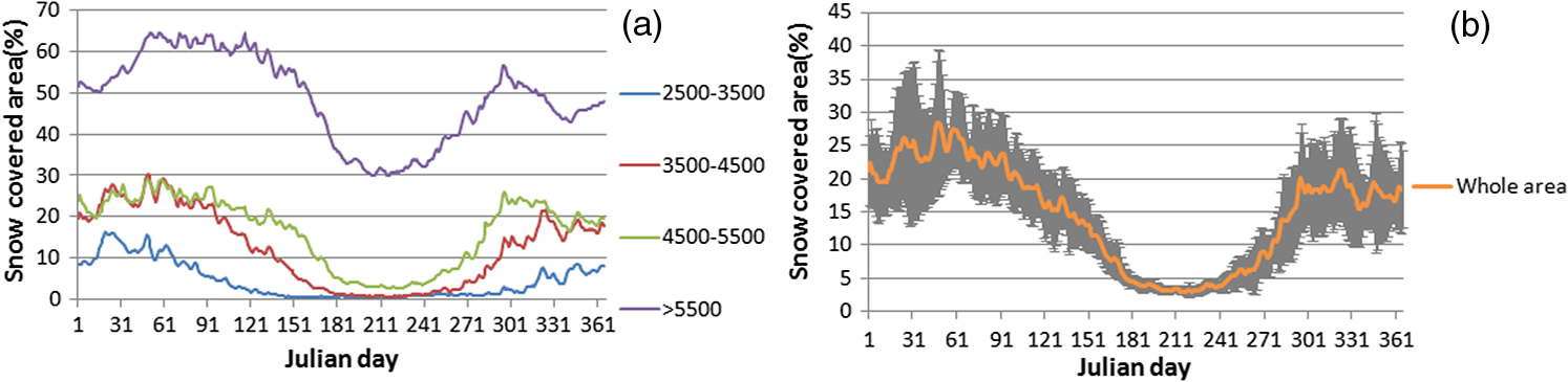

The change in the snow cover extent is almost monotonously increasing with the increasing elevation [Fig. 6(a)]. Strong seasonal variations in SCA are found over the whole area of the TP [Fig. 6(b)]. From the end of October to beginning of May, the SCA over the whole area is greater than 15% with relatively large standard deviations reflecting the very high inter-annual variability. While in the July to August period, the SCA over the whole area is less than 5% and with a relatively small inter-annual variability.

The SCA, depending upon the elevation, peaks in January at the lower elevations ( $< 3500 m$ ) and later as in March to April at elevations above 5500 m, and then progressively decreases (melts) and reaches minimum values in the July to August period [Fig. 6(a)]. In June, snow is present above 3500 m in the TP; at the lower elevations ( $< 3500 m$ ), snow is almost not present after the beginning of May. The accumulation of snow in the TP, also depending upon the elevation, starts in the beginning of September at higher elevations ( $> 5500$ ) and as late as in the end of October at elevations below 3500 m. Seen from the whole area of TP [Fig. 6(b)], the obvious snow melting and accumulation periods occur in March to June and September to October, respectively.

At elevations above 5500 m, the SCA is greater than 30% throughout the year, with two maxima in SCA appearing in spring and autumn seasons and a relatively minimum during December to January along with the typical minimum in the July to August period [Fig. 6(a)]. The relative minimum in SCA during winter months at higher elevations can be seen as the unique characteristic of snow cover in TP, which may be principally attributed to the following aspects: (1) very dry weather and less frequent snowfall during the winter months at this elevation in TP under the influence of mid-latitude cold current in winter; and (2) increased sublimation of the snow over this high-elevation area where it is frequently accompanied by high winds. More than half of the snow mass in the TP was lost by sublimation in winter.³⁶

4.4.

Characteristics of Spatial and Temporal Variations of Snow Cover

The results of SCD from 2001 to 2011 over the TP are shown in Fig. 7. The areas with SCD greater than 60 are usually considered as stable snow-cover areas in China,³⁷ and they are the major containers of snow water resources and the areas where many large rivers originate from.

Fig. 7

Distributions of MODIS derived snow-covered days (SCD) from 2001 to 2011 over the TP.

The areas with higher SCD correspond well with the huge mountains, including Kunlun, Karakoram, Himalaya, Qilian, Tanggula, and Hengduan Mountains. The most persistently SCAs (with SCD greater than 240 days) are concentrated in these huge mountain regions. In contrast, due to strong shielding from these huge mountains, most of the interior of the TP has relatively lower snow-covered persistence (with SCD less than 60 days) although the averaged elevation is over 4000 m.

For each pixel, the linear trend of SCD over the 11 years [Fig. 8(a)] and its statistical significance level [5%, Fig. 8(b)] are estimated. The linear trend analysis of SCD shows that about 34.14% of the study area has a declining trend during 2001 to 2011. However, only 5.56% pixels with a declining trend are statistically significant ( $p < 0.05$ ). Large ( $slope < - 3$ days per year) and significant ( $p < 0.05$ ) SCD decline are mainly located in the high altitude area, especially in the west of Hengduan mountains and northern Karakoram mountains. In contrast, 24.75% of pixels have an increasing trend (only 3.9% with a significant increase). Most of these pixels are located in the south of Karakoram mountains, northern Qilian mountains, and some area of the interior of the TP (between the Kunlun mountains and Tanggula mountains). About 41.11% of pixels exhibit no or very small changes (i.e., $slope < 0.5$ days per years), which are considered to be stable.

Fig. 8

Snow-covered days (SCD) trend from 2001 to 2011: (a) trend and (b) significance of trend. Trends are termed significant for pixels in which $p < 0.05$ .

Figure 9 depicts time series of the average SCD for different elevation zones and the average SCA (%) for different seasons of the whole TP during 2001 to 2011. It demonstrates that the variability of snow cover in these 11 years is characterized by normal oscillation. Snow cover fluctuates around the mean value. The time series of fluctuations in average SCD and SCA in the whole area show very high inter-annual variability, although no obvious increase or decrease tendency is found in them. For instance, the average snow cover in the TP during the spring of 2004 was only 15%, while in 2005 it was about 26%.

Fig. 9

(a) Inter-annual variation of the average snow-covered days (SCD) for different elevation zones and (b) average snow-covered area (SCA) (%) for different seasons of the whole TP from 2001 to 2011.

However, with only 11 years of MODIS data, it’s hard to reach any definitive conclusion according to the time trend of the SCD and SCA for this area. Consequently, a longer time series of data are needed to reach any definitive conclusions.

4.5.

Correlations Between Snow Cover and Temperature

Low temperature is an essential condition to meet the formation of snow cover. Moreover, rising temperature is the main reason for accelerated snow melting. To find a clue to the response of snow cover to temperature change, it is necessary to understand the linkage of variations between snow cover and temperature.

Table 3 shows the Pearson correlation coefficients between the monthly snow cover and the in situ measurements of temperature at different elevation zones. The variability of snow cover and temperature of the months (and elevation zones) with reasonably high correlation coefficients (statistical significance at the 0.01 level) are selected and shown in Fig. 10. The correlation coefficients between snow cover and temperature vary among different months and elevations, showing a large spatial and temporal heterogeneity. The snow cover in most of the months and elevations shows negative correlation with the temperature of the same month, particularly in some elevations of February, April, May, August, and September (Table 3). These high negative correlations between snow cover and temperature indicate that temperature strongly affects the snow cover.

Table 3

Pearson correlation coefficients between monthly snow cover and temperature at different elevation zones in the TP from 2001 to 2011.

Months	Elevations (m)
Months	$< 3500$	3500 to 4500	4500 to 5500	$> 5500$	Whole
Jan	$- 0.531$	$- 0.284$	$- 0.599$	$- 0.544$	$- 0.447$
Feb	$- 0.881$ **	$- 0.738$ **	$- 0.618$ *	$- 0.450$	$- 0.708$ *
Mar	$- 0.211$	$- 0.209$	$- 0.589$	$- 0.486$	$- 0.386$
Apr	$- 0.315$	$- 0.430$	$- 0.756$ **	$- 0.799$ **	$- 0.612$ *
May	$- 0.71$ *	$- 0.640$ *	$- 0.838$ **	$- 0.770$ **	$- 0.699$ *
Jun	N.A.	0.324	$- 0.134$	$- 0.389$	0.071
Jul	N.A.	N.A.	$- 0.263$	$- 0.467$	$- 0.277$
Aug	N.A.	N.A.	$- 0.810$ **	$- 0.707$ *	$- 0.795$ **
Sep	N.A.	$- 0.577$	$- 0.793$ **	$- 0.821$ **	$- 0.592$
Qct	$- 0.544$	$- 0.148$	$- 0.445$	$- 0.520$	$- 0.432$
Nov	$- 0.621$ *	$- 0.200$	$- 0.367$	$- 0.326$	$- 0.430$
Dec	$- 0.048$	0.122	$- 0.063$	$- 0.275$	0.190

Note: ** and * indicate statistical significance at the 0.01 and 0.05 level, respectively. The periods in which the snow covers are less than 2% are represented by “N.A.” (meaning “not available”).

Fig. 10

Variability of snow cover (%) and temperature in the months (and elevation zones) with reasonably high correlation coefficients (statistical significance at the 0.01 level) from 2001 to 2011.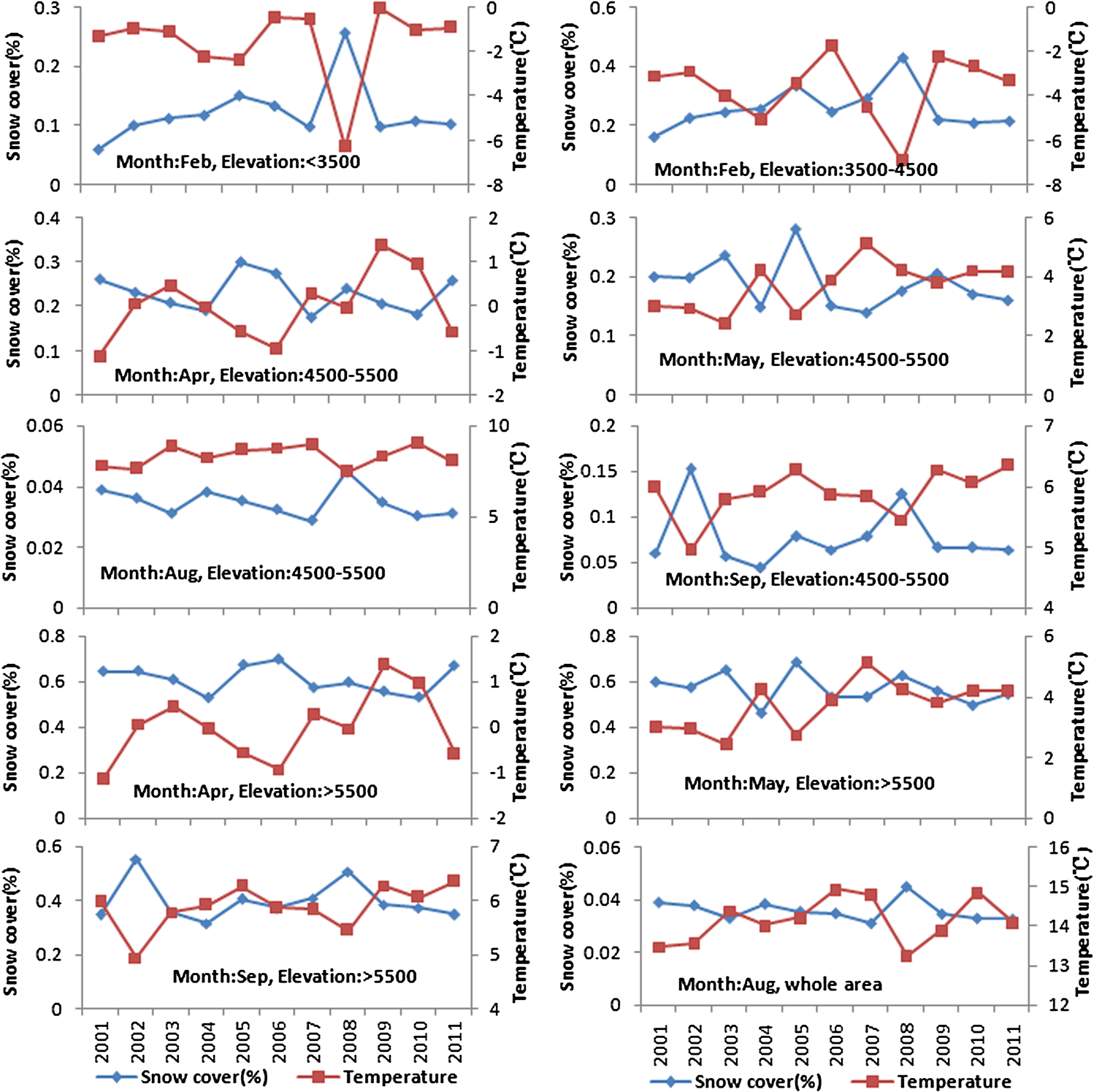

The impact of the temperature on snow cover can be explained as following two aspects. One is that the rising temperature increases the melting of snow in the snowmelt season, for example, the high negative correlations in April and May. The other is the decreasing temperature increases the snowfall in the early snowfall season, such as the high negative correlations in August and September for the high elevation zones.

Besides, snowfall is also an important influencing factor for the snow cover changes. In the TP, snowfall mainly concentrates in autumn and spring. Because of the very dry weather, there is little snowfall in winter months (especially in February). For instance, the SCA in other snow season months (such as in October, November, and March) shows a weak negative correlation with temperature, which indicates that the snowfall (as a positive factor) also greatly affects the snow cover in these months.

In winter, the influence factors of SCA are more complex, which include the small amount of snowfall and the temperature-related sublimation and melt. In December and January, because the temperature is well below the freezing over the TP, there is little temperature-related snow melting, while the temperature can also reasonably affect the SCA through changing the sublimation of snow. Besides, the small amount of snowfall also positively affects the SCA. Thus, the SCA in December and January shows a weak negative correlation with temperature. While in February, as the temperature rises, the daily maximum temperature is obviously higher than freezing in some low elevation zones, and snow begins to melt in these areas. The temperature-related snow sublimation and melt as well as the rare snowfall lead to the significant negative correlations between SCA and temperature in February.

5. Conclusions

The MODIS daily snow products (MOD10A1) from the Terra satellite have provided an excellent opportunity to analyze the spatial and temporal distribution of snow cover over the TP. The MODIS FSC data in MOD10A1 have sufficient accuracy to reflect snow cover information over the TP (with mean absolute error is about 0.098).

Based on cubic spline interpolation algorithm, the CGF method can effectively eliminate the cloud obscuration of MODIS FSC images using the observations in cloud-free days for each cloud pixel. The overall mean absolute error of the CGF method is 0.092, indicating that this method has relatively high accuracy on cloud reduction and snow information retrieval.

The most persistently SCAs are concentrated in the southern and western edges of the TP, where there are huge mountains. In the interior of the TP, snow cover is relatively small and less persistent. Moreover, there exist strong intra-seasonal variations in SCA over the TP. But the maximum snow accumulation and melting times over the year vary in different elevation ranges.

The very high inter-annual variability of SCD and SCA during 2001 to 2011 is discovered. About 34.14% (5.56% with a significant decline) and 24.75% (3.9% with a significant increase) of the study area shows declining and increasing trend in SCD, respectively. However, a longer time series of data need to be examined to obtain some definitive conclusions about temporal trends. Some of the inter-annual fluctuation of snow cover can be explained by the high negative correlations which are observed between the snow cover and in situ air temperature. If global warming goes on, the decrease of snow cover caused by the high negative correlation with temperature in February, April, and May, may result in significant changes in the river flows and water resources in the TP, particularly in spring. This will have impacts on ecosystem, irrigation dependent agriculture, and water resources in the densely populated downstream areas.

Acknowledgments

This study was supported by the National Basic Research Program of China (grant no. 2010CB951403), the National Natural Science Foundation of China (grant no. 41071227), the National Natural Science Foundation of China (Grant No. 91025001), and the FP7 project “CEOP-AEGIS” (Grant No. 212921).

References

1.

J. L. Fosteret al., “Quantifying the uncertainty in passive microwave snow water equivalent observations,” Remote Sens. Environ., 94 (2), 187 –203 (2005). http://dx.doi.org/10.1016/j.rse.2004.09.012 RSEEA7 0034-4257 Google Scholar

2.

J. Dozieret al., “Time-space continuity of daily maps of fractional snow cover and albedo from MODIS,” Adv. Water Resour., 3 (11), 1515 –1526 (2008). http://dx.doi.org/10.1016/j.advwatres.2008.08.011 AWREDI 0309-1708 Google Scholar

3.

J. WangS. Li, “Effect of climate change on snowmelt runoffs in mountainous regions of inland rivers in northwestern china,” Sci. China Ser. D, 49 (8), 881 –888 (2006). http://dx.doi.org/10.1007/s11430-006-0881-8 SCDEF8 1006-9313 Google Scholar

4.

J. F. LiuR. S. Chen, “Studying the spatiotemporal variation of snow-covered days over China based on combined use of MODIS snow-covered days and in situ observations,” Theor. Appl. Climatol., 106 (3–4), 355 –363 (2011). http://dx.doi.org/10.1007/s00704-011-0441-9 TACLEK 1434-4483 Google Scholar

5.

J. Qiu, “The third pole,” Nature, 454 (24), 393 –396 (2008). http://dx.doi.org/10.1038/454393a NATUAS 0028-0836 Google Scholar

6.

B. T. PanJ. J. Li, “Qinghai-Tibetan plateau: a driver and amplifier of the global climatic change,” J. Lanzhou Univ., 32 108 –115 (1996). Google Scholar

7.

X. D. Liuet al., “Temporal trends and variability of daily maximum and minimum, extreme temperature events, and growing season length over the eastern and central Tibetan Plateau during 1961–2003,” J. Geophys. Res., 111 D19109 (2006). http://dx.doi.org/10.1029/2005JD006915 JGREA2 0148-0227 Google Scholar

8.

Y. F. ShiY. P. ShenR. J. Hu, “Preliminary study on signal, impact and foreground of climatic shaft from warm-dry to warm-wet in Northwest China.,” J. Glaciol. Geocryol., 24 (3), 219 –226 (2002). 1000-0240 Google Scholar

9.

Y. F. Shiet al., “Recent and future climate change in northwest China,” Clim. Change, 80 (3–4), 379 –393 (2007). http://dx.doi.org/10.1007/s10584-006-9121-7 CLCHDX 0165-0009 Google Scholar

10.

X. Liet al., “Cryospheric change in China,” Global Planet Change, 62 (3–4), 210 –218 (2008). http://dx.doi.org/10.1016/j.gloplacha.2008.02.001 GPCHE4 0921-8181 Google Scholar

11.

S. C. Kanget al., “Review of climate and cryospheric change in the Tibetan plateau,” Environ. Res. Lett., 5 015101 (2010). http://dx.doi.org/10.1088/1748-9326/5/1/015101 ERLNAL 1748-9326 Google Scholar

12.

D. H. QinY. J. Ding, “Cryospheric changes and their impacts: present, trends and key issues,” Adv. Clim. Change Res., 5 (4), 187 –195 (2009). 1673-1719 Google Scholar

13.

Z. X. PuL. XuV. V. Salomonson, “MODIS/Terra observed seasonal variations of snow cover over the Tibetan Plateau,” Geophys. Res. Lett., 34 (6), L06706 (2007). http://dx.doi.org/10.1029/2007GL029262 GPRLAJ 0094-8276 Google Scholar

14.

P. J. Li, “Response of Tibetan snow cover to global warming,” Acta Geographica Sinica, 51 (3), 260 –265 (1996). 0375-5444 Google Scholar

15.

Z. G. Wei, “Snow cover data on Qinhai Xizang Plateau and its correlation with summer rainfall in China,” Q. J. Appl. Meteorol., 9 39 –46 (1998). Google Scholar

16.

W. J. DongZ. G. WeiL. J. Fan, “Climatic character analyses of snow disasters in East Qinghai-Xizang Plateau livestock farm,” Plateau Meteorol., 20 (4), 402 –406 (2001). Google Scholar

17.

Y. ZhangT. LiB. Wang, “Decadal change of the spring snow depth over the Tibetan Plateau: the associated circulation and its influence on the East Asian summer monsoon,” J. Clim., 17 2780 –2793 (2004). http://dx.doi.org/10.1175/1520-0442(2004)017<2780:DCOTSS>2.0.CO;2 JLCLEL 0894-8755 Google Scholar

18.

Z. W. Wanget al., “Research progress of satellite data utilization for snow monitoring in pastoral areas,” Pratacult. Sci., 26 (1), 32 –39 (2009). Google Scholar

19.

Y. C. BaiX. Z. Feng, “Introduction to some research work on snow remote sensing,” Remote Sens. Technol. Appl., 12 (2), 59 –65 (1994). Google Scholar

20.

D. K. Hallet al., “MODIS snow-cover products,” Remote Sens. Environ., 83 (1–2), 181 –194 (2002). http://dx.doi.org/10.1016/S0034-4257(02)00095-0 RSEEA7 0034-4257 Google Scholar

21.

D. K. HallG. A. Riggs, “Accuracy assessment of the MODIS snow products,” Hydrol. Process., 21 1534 –1547 (2007). http://dx.doi.org/10.1002/(ISSN)1099-1085 HYPRE3 1099-1085 Google Scholar

22.

M. RodellP. R. Houser, “Updating a land surface model with MODIS derived snow cover,” J. Hydrometeorol., 5 (6), 1064 –1075 (2004). http://dx.doi.org/10.1175/JHM-395.1 1525-755X Google Scholar

23.

J. Parajkaet al., “A regional snow-line method for estimating snow cover from MODIS during cloud cover,” J. Hydrol., 381 (3–4), 203 –212 (2010). http://dx.doi.org/10.1016/j.jhydrol.2009.11.042 JHYDA7 0022-1694 Google Scholar

24.

D. K. Hallet al., “Snow cover, snowmelt timing and stream power in the Wind River Range, Wyoming,” Geomorphology, 137 (1), 87 –93 (2012). http://dx.doi.org/10.1016/j.geomorph.2010.11.011 GMPHAA 0169-555X Google Scholar

25.

J. ParajkaG. Blöschl, “Spatio-temporal combination of MODIS images-potential for snow cover mapping,” Water Resour. Res., 44 (3), W03406 (2008). http://dx.doi.org/10.1029/2007WR006204 WRERAQ 0043-1397 Google Scholar

26.

Y. Gaoet al., “Integrated assessment of multi-temporal and multi-sensor combinations for reducing cloud obscuration of MODIS snow cover products for the Pacific Northwestern USA,” Remote Sens. Environ., 114 (8), 1662 –1675 (2010). http://dx.doi.org/10.1016/j.rse.2010.02.017 RSEEA7 0034-4257 Google Scholar

27.

H. XieX. WangT. Liang, “Development and assessment of combined Terra and Aqua snow cover products in Colorado Plateau, USA and northern Xinjiang, China,” J. Appl. Remote Sens., 3 (1), 033599 (2009). http://dx.doi.org/10.1117/1.3265996 Google Scholar

28.

X. WangH. Xie, “New methods for studying the spatiotemporal variation of snow cover based on combination products of MOIDS Terra and Aqua,” J. Hydrol., 371 (1–4), 192 –200 (2009). http://dx.doi.org/10.1016/j.jhydrol.2009.03.028 JHYDA7 0022-1694 Google Scholar

29.

T. G. Lianget al., “Toward improved daily snow cover mapping with advanced combination of MODIS and AMSR-E measurements,” Remote Sens. Environ., 112 (10), 3750 –3761 (2008). http://dx.doi.org/10.1016/j.rse.2008.05.010 RSEEA7 0034-4257 Google Scholar

30.

Y. Gaoet al., “Toward advanced daily cloud-free snow cover and snow water equivalent products from Terra-Aqua MODIS and Aqua AMSR-E measurements,” J. Hydrol., 385 (1–4), 23 –35 (2010). http://dx.doi.org/10.1016/j.jhydrol.2010.01.022 JHYDA7 0022-1694 Google Scholar

31.

D. K. Hallet al., “Development and evaluation of a cloud-gap-filled MODIS daily snow-cover product,” Remote Sens. Environ., 114 (3), 496 –503 (2010). http://dx.doi.org/10.1016/j.rse.2009.10.007 RSEEA7 0034-4257 Google Scholar

32.

Y. GaoN. LuT. D. Yao, “Evaluation of a cloud-gap-filled MODIS daily snow cover product over the Pacific Northwest USA,” J. Hydrol., 404 (3–4), 157 –165 (2011). http://dx.doi.org/10.1016/j.jhydrol.2011.04.026 JHYDA7 0022-1694 Google Scholar

33.

V. V. SalomonsonI. Appel, “Estimating the fractional snow covering using the normalized difference snow index,” Remote Sens. Environ., 89 (3), 351 –360 (2004). http://dx.doi.org/10.1016/j.rse.2003.10.016 RSEEA7 0034-4257 Google Scholar

34.

G. A. RiggsD. K. HallV. V. Salomonson, “MODIS Snow Products User Guide Collection 5,” (2006) http://modis-snow-ice.gsfc.nasa.gov/sugkc2.html Google Scholar

35.

“MODIS Reprojection Tool (MRT), 2008. User’s manual, release 4.0,” https://lpdaac.usgs.gov/lpdaac/content/&hell:/MRT_Users_Manual.pdf Google Scholar

36.

D. H. QinS. Y. LiuP. J. Li, “Snow cover distribution, variability, and response to climate change in western China,” J. Clim., 19 (9), 1820 –1833 (2006). http://dx.doi.org/10.1175/JCLI3694.1 JLCLEL 0894-8755 Google Scholar

37.

P. J. LiD. S. Mi, “Distribution of snow cover in China,” J. Glaciol. Geocryol., 5 9 –17 (1983). Google Scholar

Biography

Biographies and photographs of the authors are not available.

CC BY: © The Authors. Published by SPIE under a Creative Commons Attribution 4.0 Unported License. Distribution or reproduction of this work in whole or in part requires full attribution of the original publication, including its DOI.

Citation Download Citation

Zhiguang Tang, Jian Wang, Hongyi Li, and Lili Yan "Spatiotemporal changes of snow cover over the Tibetan plateau based on cloud-removed moderate resolution imaging spectroradiometer fractional snow cover product from 2001 to 2011," Journal of Applied Remote Sensing 7(1), 073582 (4 March 2013). https://doi.org/10.1117/1.JRS.7.073582

Published: 4 March 2013

Access the abstract

JOURNAL ARTICLE
15 PAGES

DOWNLOAD PAPER SAVE TO MY LIBRARY

GET CITATION

CITATIONS

Cited by 97 scholarly publications.

Explore citations on Lens.org

KEYWORDS

Snow cover

MODIS

Single crystal X-ray diffraction

Clouds

Earth observing sensors

Landsat

Binary data

1.

Introduction

2.

Study Area