|
|
1.IntroductionNatural disasters occur all over the world. They can happen anywhere at any time. In Europe, floods are the most frequent type of natural disaster and account for 75% of all insurance claims arising from natural disasters.1 Administration organizations work before, during, and after the crisis events to issue alerts, monitor events, and estimate the impact. Real damage evaluations carried out after the disaster allow for the verification and improvement of model calculations. Satellite images have increased the ability to assess and predict natural hazards, and this helps prevent the loss of property, infrastructure, and human lives. Since 2000, a number of spaceborne satellites and sensors have changed the way we assess and predict natural disasters. These sensors can quantify geophysical phenomena associated with natural hazards. Significant improvements in the near real-time assessments of natural hazards have been made due to increased data acquisition rates, higher sensor resolution, the improvement of change detection algorithms, and the integration of remote sensing systems.2 However, natural disasters will never become completely predictable. They keep occurring, the affected areas must be detected, and damage assessment still must be performed. In recent years, Slovenia has been hit by numerous floods. The largest flood events occurred in September 2007 and September 2010. The first one devastated the area covered by the municipalities of Železniki, Bohinj, Cerkno, and Idrija.3 The second devastated a third of Slovenia;4 central Slovenia and the capital of Ljubljana were hit the worst. This paper deals with the 2007 event. The weather front that passed over the impact area in a matter of hours yielded enough rainfall to cause severe flash floods in several parts of Slovenia.5 Since the flash flooding was most intense in the area surrounding the town of Železniki, our analysis focused on this part of the flooded valley. The event caused colossal material damage. Several villages were completely cut off, and several people died. In such cases, rescue teams need to know the current situation in the field. This information can be best mediated if the affected area is mapped in real time. Our procedure assures rapid and accurate mapping using machine learning techniques. Having readily available input data from various sources for machine learning is a precondition for fast mapping. Satellite images, digital terrain models (DTMs), and the river network were used in our example. The output is a classification model for detecting flooded areas. A number of models were built using different machine learning algorithms, all of which were tested in various conditions (data input resolution and training set samples). The effectiveness of each algorithm was tested with randomly generated testing points and stratified cross-validation. The model with the best classification results was chosen for use on a broader area. 2.DataSatellite images provided the main data for flood area detection with machine learning procedures. These are appropriate for flood observations, because they can cover large areas quickly. However, their limitations could be found in their spatial and temporal resolution (a rapid image sequence is desirable) and sometimes in their inadequate spectral bands. For best results, satellite data should be supplemented with other sources, such as DTMs and hydrology. This data will offer numerous additional attributes that can be used to improve flood determination. In our experiments, we used the mentioned data as attributes in machine learning (Table 1). Table 1Attributes of the input data used for machine learning processes.
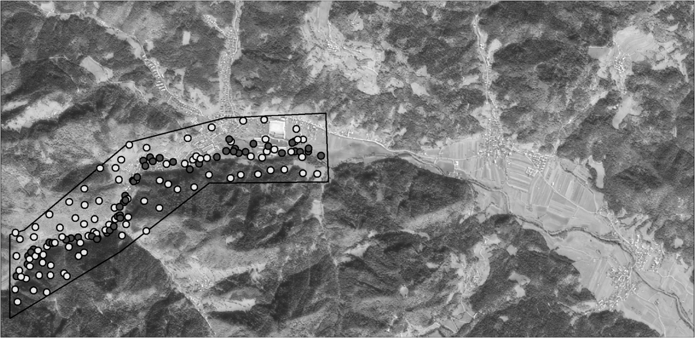
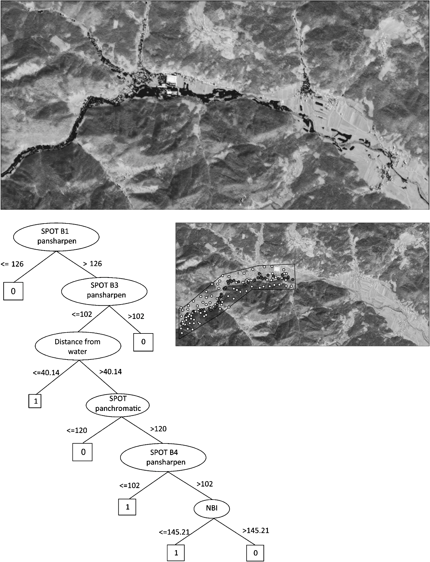
SPOT 5 satellite images were obtained in panchromatic mode at 2.5-m resolution and in multispectral mode at 10-m resolution. Images were acquired within the frame of International Charter Space and Major Disaster,6 which, in the event of any natural or manmade disaster, provides access to free satellite images and products in the shortest possible time. The SPOT 5 images were acquired three days after the disaster, i.e., on 21 September 2007, when the clouds moved away from the affected area. Because the flash flooding was triggered by torrential rain that fell over a very short period (approximately two hours), it was hard to observe with any satellite system. It would be difficult to obtain images in such a short time, and therefore only the consequences of the floods and wet areas can be observed. The resolution of the multispectral image was increased from 10 m to 2.5 m by pan-sharpening. To initiate the process, multispectral images of both resolutions were used (Table 1). Various combinations of satellite image bands (red, near infrared, and shortwave infrared) were used to calculate indexes; we selected normalized difference vegetation index (NDVI), normalized difference built-up index (NDBI), and new built-up index (NBI) for machine learning.7 Since rapid mapping was given priority over accuracy, the images were not calibrated or radiometrically corrected. Consequently, the indexes do not represent their true value. Anyway, in a case where the index values are limited to a single study, such behavior is acceptable. We are currently developing an automatic image processing chain (including geometric and radiometric corrections) that will enable us to assure operability of the procedure on any image.8 The indexes were calculated as The NDVI was used to separate flooded areas from vegetation. The two other indexes were used to detect built-up areas. Height, slope, and aspect were derived from DTMs at two different resolutions: the national DTM at 12.5 m and the laser scanning (lidar)-based DTM at 0.5 m. Lidar points were recorded only for the area that was most damaged by the floods, and consequently the area under analysis was decreased to this area (marked by the black border on Fig. 1). Hydrology was used to calculate the distances from the rivers. The digital topographic map of the river network with a 1:25,000 scale was used. 3.MethodologyIt is hard to identify flooded areas from satellite images. Cloud cover often affects or even limits the use of optical imagery. On the other hand, radar waves can penetrate cloud cover, and their temporal resolutions do not lag too far behind the resolution of optical imagery. The latest constellation of satellites equipped with SAR sensors, (e.g., COSMO-SkyMed) enable repeat observations several times a day,9 and TerraSAR-X enables observations every two days.10 Both radar satellites provide high-resolution SAR imagery with a resolution of up to 1 m. In our case, ENVISAT and RADARSAT images were acquired for the flooded area of Železniki, but they proved unsuitable, because the rough terrain makes some parts of the valley invisible to the sensor (i.e., the bottom is affected by shadows). Another problem was the fast water outflow after the event and the need to recognize mud and other material deposits. Similar electromagnetic properties measured by satellite sensors in different types of land produce misclassifications. For example, the SPOT panchromatic band does not distinguish between fields and pastures, and none of the SPOT multispectral bands distinguish with certainty between flooded and built-up areas.11 Therefore, we tried to improve the detection of flooded areas with the use of additional data and different machine learning algorithms, including ensembles. As a result of the machine learning process, we came up with a model. This very complex model fits the training data perfectly. However, overfitted models set to the training data are not good. The model should be robust enough to be applicable to a broader area. To extract flooded areas, we tested different methods involving two machine learning software packages: Weka12 and Clus.13 3.1.Testing the Impact of Training SetsTwo different sizes of training sets with the same attributes were tested. Some experience in learning with different numbers of training points has already been gained. However, the number of training points and the treated area were increasing proportionally in our case, so the correctness of the classification did not increase with the number of training points.14 The learning process did not benefit from additional points, because they did not contribute any new information about the flooded area. This time we used 255 learning points arranged throughout the entire area (Fig. 2), as well as 145 learning points arranged across a smaller part of the studied area (Fig. 1). The smaller area coincides with the area covered by DTM 0.5. In both areas, the training points were arranged randomly. However, a few points in the smaller training set were displaced slightly in order to achieve higher representation. Algorithm J48 and DTM 12.5 were used to test the influence of the different numbers of learning points. The accuracy of the classification was 85.6% when the smaller area with 145 training points was used and 80.8% when the entire area with 255 training points was used. This shows that the sampling points should be chosen with great care. The point density was higher in the training examples of the smaller area. A higher density of points and their arrangement in heterogeneous surfaces with different types of land cover assure that the different characteristics of the area are included in the training data set. In this way, the flooded area is better represented, especially when we are dealing with a heterogeneous landscape. In our case, the points were located in urban areas, flooded fields, flooded meadows, forests, etc. The selection of training points in heterogeneous areas was assured by digital orthophoto. The definition of flooded and unflooded training points was based on the visual interpretation of the satellite images, hydraulic measurements, and field observations immediately after the torrential rain. The importance of the sample data sets can be illustrated by the example of buildings. The points located on the roofs of buildings have to be explicitly determined as unflooded; otherwise, disturbances between flooded and built-up areas can occur, due to their similar reflection of radiation in SPOT multispectral bands.9 Fig. 2Sample of 255 training points arranged throughout the entire treated area. Dark points represent flooded locations.  Additionally, we have used the object-based approach and replaced the training points with training segments (Fig. 3). These segments are groups of pixels with common spectral, geometrical, and textural characteristics that represent real geographical objects.4 In our case, the segmentation rate was very small, so each segment does not represent an individual object. In the case of segments, the attributes are computed as an average value for a segment area. Fig. 3Training sample with segments. We used 256 segments for the entire area and 143 segments for the smaller part. Only segments that were used for learning are shown here. 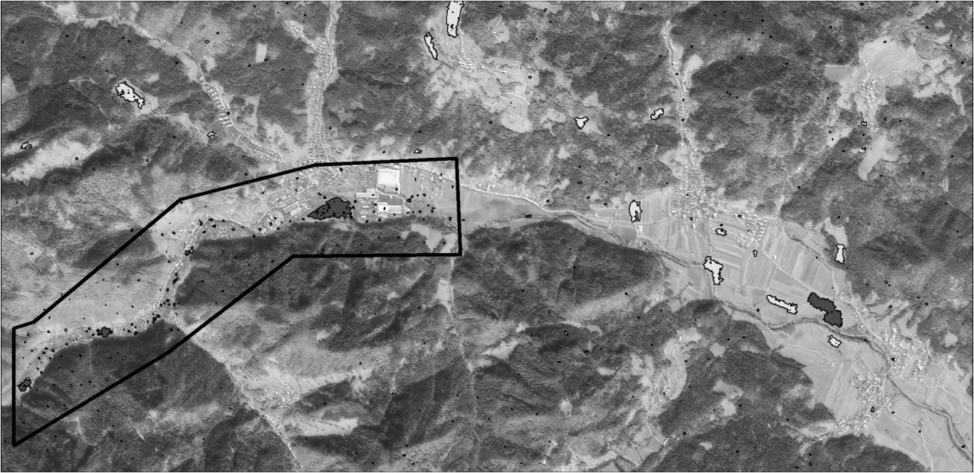 The comparison of classification with points and segments was performed for a smaller area. The test with 100 points did not confirm that learning based on segments would add anything to the classification. When the learning data set consisted of 145 training points, 95% of the testing points were classified correctly, while 91% accuracy was achieved when 143 training segments replaced the 145 training points. 3.2.Testing the Influence of DTM ResolutionIn the next step, the training set of 145 training points (Fig. 1) was tested in relation to DTM 0.5 and DTM 12.5 m. All samples consisted of attributes derived from the same data sets: satellite images, DTMs, and the river network (see Sec. 2). The only difference during testing was the DTM resolution. Heights, slopes, and aspects were derived from the DTM with resolutions of 0.5 m and 12.5 m. The learning with attributes derived from DTMs with both resolutions was performed with the J48 algorithm, with which we determined the difference in classification. This showed that a higher DTM resolution does not contribute significantly to an improved classification of flooded areas. The detection rates for flooded areas are similar in both examples; 95% of the testing points were classified correctly in the first example, and 92% were classified correctly in the second example. Figure 4 shows that only slope was included in the model built by DTM 0.5 (a), while no attribute derived from DTM 12.5 was included (b). Other attributes (height and aspect) evidently do not contribute to the classifications. This relates to the characteristics of the studied alpine valley. Its lower part sweeps gently down to the end, and areas with very different heights and aspects are flooded. The upper parts of the decision trees are identical in the DTM 0.5 and DTM 12.5 classifications. In the lower part, the SPOT panchromatic band replaces the slope attribute derived from DTM 0.5, and two additional nodes are added to the model on the right (Fig. 4). This makes the classification chart on DTM 12.5 larger and more complex. 3.3.Testing Classification AlgorithmsIn our next test, we investigated several classification algorithms (Table 2), including some that cannot be used to create classification models. One of them was the Naive Bayes classifier, which is a probabilistic classifier. The Naive Bayes probability model cannot be used in our case, because we have a small number of outcome classes (two) and a large number of features (16), which can take on a lot of different values. In the end, we tested those machine learning methods that seemed to be the most suitable for the classification of flooded areas with two classes (flooded and unflooded areas). In relation to the small testing area, the classification methods using DTM 0.5 and 145 training points were used. In Weka, the following classifier algorithms were examined: the J48 decision tree algorithm,15,16 the JRip rule induction algorithm,17 and the Bagging meta-learning algorithm,18 which generated a diverse ensemble of classifiers. The Bagging ensemble method in Weka was compared to the Random Forest19 method in the CLUS machine learning software. Ensembles with different numbers of trees were produced. Table 2Machine learning algorithms tested for flood detection. Algorithms marked with an asterisk were proven to be the most suitable for flood classification in our case study.
Following successful machine learning, the classification models were prepared, and maps of flooded areas were produced. 4.Results4.1.Comparison of Classifications with Different Data InputClassifications with different numbers of training points and different DTM resolutions have proven that the sample of 145 training points and attributes derived from DTM 0.5 produce the best results. The results derived from the attributes obtained by DTM 0.5 were slightly better than those obtained by DTM 12.5. The classification tree in the case of DTM 12.5 is also larger and too complex to use in the classification of a broader area. 4.2.Evaluation of Machine Learning ClassifiersTable 3 shows the accuracy evaluation results for each method. The training success with each machine learning method is presented with the percentage of correctly classified training points. Ten-fold cross validation was used to define the percentage of correctly classified training points. Randomly generated testing points were used to assess the accuracy of the final maps of the flooded area. Table 3Accuracy of flood detection using various machine learning methods. Among ensembles with different numbers of trees, those with 10 trees are presented in the table, because they were shown to be optimal.
The decision tree is a practical form of the model in which we deal with a binary classification in which only two classes are possible: flooded and unflooded areas. The highest classification accuracy measured by randomly generated testing points was obtained by the single tree J48 algorithm (95%). Classification accuracy of 92% was obtained by ensemble algorithms (Bagging, Random Forest), while 85% classification accuracy was obtained by the JRip rules algorithm. Similar algorithms were used to build an ensemble of models. We expected an improvement in the classifications, but this did not happen. The accuracy of the ensemble methods did not exceed the accuracy of the single model. An ensemble of size 10 already reaches a high accuracy value, which cannot be significantly increased by increasing the number of trees (Table 4). Table 4Accuracy of flooded area detection with the use of the Random Forest method (CLUS). Comparison of classifications with different numbers of trees.
The higher accuracy of testing points (when compared to training points) is a consequence of the locality of training points, some of which were arranged in areas that are hard to classify (e.g., points located on rooftops are unflooded). However, it could be difficult to extract these unflooded areas from the flooded areas surrounding them. Similar examples are points lying on a riverbank overgrown by trees and shrubs. These points should be denoted as flooded if water could be detected through the plants or unflooded if the canopy covers the surface completely. Such selection of training points makes it possible to produce a good classification, although randomly generated testing points can achieve even higher accuracy. 4.3.Mapping of the Flooded AreaFigure 5 shows the flooded area detected by the J48 algorithm (a). The maps generated by other models are not presented, because they are visually similar. This figure clearly indicates that the misclassifications occur mostly in built-up areas and fields. Both areas are presented in similar tones in Fig. 5. Misclassifications were a result of similar reflections of radiation from flooded and unflooded built-up areas or fields. The classification model is shown on the right side of the figure; it was built on training data of 145 points and consists of four nodes and five leaves. The attributes that take part in this classification are the green and near IR bands of the SPOT pan-sharpened image, distance from water, and slope. It is seen that the three indexes calculated from different bands of SPOT multispectral image were not included in the model. However, the green and near IR bands could replace the NDVI index to detect vegetation. NDBI and NBI were evidently incapable of recognizing built-up areas in the treated area. Fig. 5Map of the flooded area detected by Weka’s J48 learning algorithm on 145 training points. (a) Flooded areas are shown in dark. (b) The classification tree is shown on the right part of the figure. The slope attribute was derived from DEM with a resolution of 0.5 m. 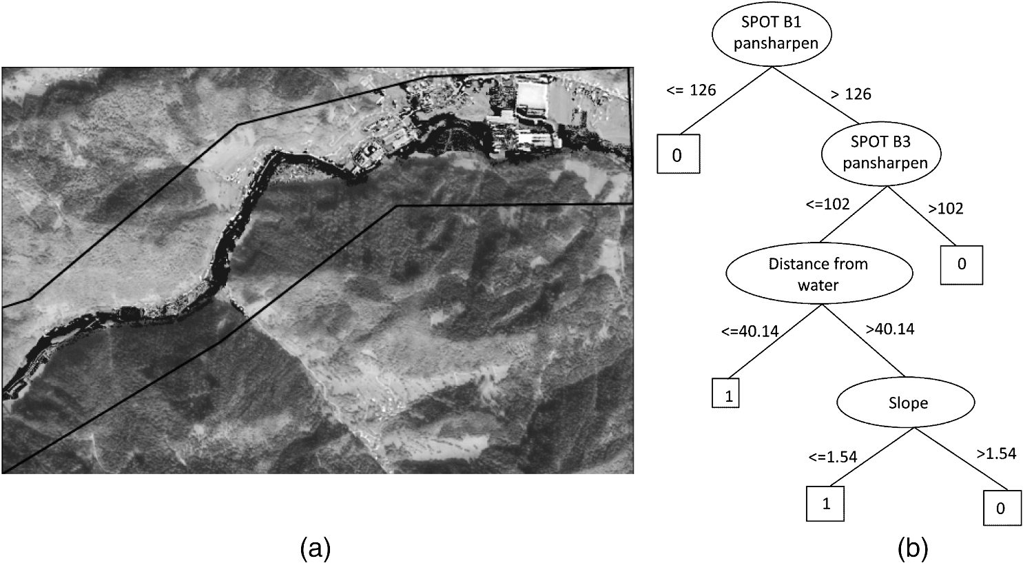 The produced model should be robust enough to be applied to any flood event in an area with similar characteristics. For this reason, the model generated in the training area was applied for classification in a larger area (Fig. 6). The training area, the number of training points, and their attributes were the same as in the previous example, but DTM 0.5 was replaced by DTM 12.5. The accuracy test showed that 85.6% of the 125 testing points arranged over the whole area were classified accurately. This confirms that our model could be used successfully outside the training area and is applicable to similar or next flood events. 5.ConclusionsIn this study, we have tested machine learning techniques used in the process of flood detection. The results have proved that the machine learning algorithms could be used for detecting flooded areas with high accuracy. To achieve accurate results, both good-quality data and an effective machine learning algorithm are essential. At first, the attributes of the training points were collected. This step is extremely important, because the success of the learning phase is highly dependent on it. High temporal and spatial data resolution are the key factors when dealing with flood monitoring. In particular, Earth observation data (satellite images) must be accessible as soon as possible after the disaster, and the spatial resolution has to be appropriate in order to observe the required flood details. The boundaries of the flooded areas can be detected only if the spatial precision of the data is high enough. To compare the classification accuracies, we used several machine learning algorithms. Among the tested set of classifiers, the J48 algorithm has proven the most successful (Table 3). This is the optimal choice for binary classifications, in which only two classes are possible: flooded or unflooded areas. Ensemble methods were also used to obtain better predictive performance. However, they did not lead to a better classification. The machine learning approach has proven very successful for flood detection and has provided accurate classification models. The percentage of accurately classified training points reaches almost 90%, and the accuracy of the final classification surpasses 90% (Table 3). However, additional input data and machine learning algorithms still need to be tested if we wish to find the best combination for detecting flooded areas. Especially problematic are built-up areas or fields, where it is hard to distinguish between flooded and unflooded areas. This aspect needs to be addressed in the future. ReferencesH. Bachet al.,
“Application of satellite data for flood monitoring,”
in Proc. GGRS,
(2004). Google Scholar
T. W. Gillespieet al.,
“Assessment and prediction of natural hazards from satellite imagery,”
Prog. Phys. Geog., 31
(5), 459
–470
(2007). http://dx.doi.org/10.1177/0309133307083296 PPGEEC 0309-1333 Google Scholar
P. Pehaniet al.,
“Uporaba satelitskih posnetkov za analizo poplav septembra 2007,”
Geografski Informacijski Sistemi v Sloveniji 2007–2008, 117
–128 Geografski Inštitut Antona Melika ZRC-SAZU, Ljubljana
(2008). Google Scholar
T. Veljanovskiet al.,
“Flooded areas determination using radar satellite images in Slovenia,”
in Proc. 7th Conf. Image Information Mining: Geospatial Intelligence from Earth Observation,
141
–144
(2011). Google Scholar
S. RusjanM. KoboldM. Mikoš,
“Characteristics of the extreme rainfall event and consequent flash floods in W Slovenia in September 2007,”
Nat. Hazards Earth Sys. Sci., 9
(3), 947
–956
(2009). http://dx.doi.org/10.5194/nhess-9-947-2009 1561-8633 Google Scholar
A. Mahmoodet al.,
“An overview of the International Charter ‘Space and Major Disasters’,”
in Geoscience and Remote Sensing Symposium, IGARSS ’02,
771
–773
(2002). Google Scholar
Y. ZhaJ. GaoS. Ni,
“Use of normalized difference built-up index in automatically mapping urban areas from TM imagery,”
Int. J. Rem. Sens., 24
(3), 583
–594
(2003). http://dx.doi.org/10.1080/01431160304987 IJSEDK 0143-1161 Google Scholar
K. Oštiret al.,
“Prototype of an automatic near-real-time satellite image processing chain,”
in Small Satellites Systems and Services Symposium, 2012 4S Symposium,
1
–14
(2012). Google Scholar
N. Pierdiccaet al.,
“Lessons learned from using COSMO-SkyMed imagery for flood mapping: some case studies,”
Proc. SPIE, 8536 85360W
(2012). http://dx.doi.org/10.1117/12.977646 PSISDG 0277-786X Google Scholar
L. Giustariniet al.,
“A change detection approach to flood mapping in urban areas using terraSAR-X,”
IEEE Trans. Geosci. Rem. Sens., 51
(4), 2417
–2430
(2013). http://dx.doi.org/10.1109/TGRS.2012.2210901 IGRSD2 0196-2892 Google Scholar
Ž. Kokaljet al.,
“Observation of torrential rains devastation in Slovenia,”
in Proc. 1st Int. Conf. Remote Sensing Techniques in Disaster Management and Emergency Response in the Mediterranean Region,
181
–190
(2008). Google Scholar
M. Hallet al.,
“The WEKA data mining software: an update,”
SIGKDD Explorations, 11
(1), 10
–18
(2009). http://dx.doi.org/10.1145/1656274 1931-0145 Google Scholar
D. Kocevet al.,
“Tree ensembles for predicting structured outputs,”
Pattern Recogn., 46
(3), 817
–833
(2013). http://dx.doi.org/10.1016/j.patcog.2012.09.023 Google Scholar
P. LamovecK. Oštir,
“Uporaba strojnega učenja za določitev poplavljenih območij—primer poplav v Selški dolini leta 2007,”
Geodetski vestnik, 54
(4), 673
–687
(2010). Google Scholar
J. R. Quinlan,
“Learning with continuous classes,”
in Proc. 5th Australian Joint Conf. Artificial Intelligence,
343
–348
(1992). Google Scholar
I. H. WittenE. Frank, Data Mining: Practical Machine Learning Tools and Techniques, 2nd ed.Morgan Kaufmann, San Francisco
(2005). Google Scholar
W. W. Cohen,
“Fast effective rule induction,”
in Proc. 12th Int. Conf. Machine Learning,
115
–123
(1995). Google Scholar
L. Breiman,
“Bagging predictors,”
Mach. Learn., 24
(2), 123
–140
(1996). http://dx.doi.org/10.1023/A:1018054314350 MALEEZ 0885-6125 Google Scholar
L. Breiman,
“Random forests,”
Mach. Learn., 45
(1), 5
–32
(2001). http://dx.doi.org/10.1023/A:1010933404324 MALEEZ 0885-6125 Google Scholar
Biography Peter Lamovec received his BSc in Geodesy from University of Ljubljana. Primarily he was involved in GIS-based environmental studies. He is currently researcher at the Research Centre of the Slovenian Academy of Sciences and Arts and PhD student on University of Ljubljana. Much of his research over the last 4 years has focused on remote sensing in natural disasters. In his PhD thesis he works on flooded areas determination using satellite images and machine learning techniques.  Tatjana Veljanovski received her BSc and PhD in geodesy from Faculty of Civil and Geodetic Engineering, University of Ljubljana. She graduated in the field of GIS-based spatial analysis for archaeological potential modelling and accomplished the postgraduate study in remote sensing. She is currently research fellow at the Research Centre of the Slovenian Academy of Sciences and Arts and at the Centre of Excellence Space-SI. Her main research fields are optical satellite and aerial remote sensing and image processing. In particular she has performed research in geometric and radiometric image pre-processing, classification, change detection and interpretation of spatial patterns. The applications of remote sensing range from hazard monitoring and mapping, landscape and urban analysis to change detection. Recently she has worked on object-based image analysis, slum-like areas identification and historical aerial image geometric restitution.  Matjaž Mikoš is the dean of the Faculty of Civil and Geodetic Engineering, University of Ljubljana, professor of hydraulic engineering and professor of hydrology. He was previously with the Water Management Institute in Ljubljana, Slovenia. He received his Diploma degree and MS degree in civil engineering from the University in Ljubljana, and his PhD degree in civil engineering from the ETH Zürich in 1993. He conducts research in applied hydrology, flood, torrent and landslide control, river engineering and river morphology, and risk management in mountainous areas.  Krištof Oštir received his PhD in remote sensing from University of Ljubljana. His main research fields are optical and radar remote sensing and image processing. In particular he has performed research in radar interferometry, digital elevation production, land use and land cover classification, post-processing and fuzzy classification. The applications of remote sensing range from hazard monitoring change detection, archaeological site analysis to paleo-environment and paleo-relief modelling. He is active in the development of small satellites for Earth observation. He is employed at the Scientific Research Centre of the Slovenian Academy of Sciences and Arts, Centre of Excellence for Space Sciences and Technologies, and as an associate professor at the University of Ljubljana, where he teaches several courses on remote sensing and satellite image processing. |
|||||||||||||||||||||||||||||||||||||||||||||||||||||||||||||||||||||||||||||||||||||||||||||||||||||||