Contoured window correlation interferometry for synthetic aperture radar interferometry based on three parts of complex images

Jianhua Shi; Sihua Fu; Xuejun Long; Xia Yang; Qifeng Yu

doi:10.1117/1.JRS.7.073559

22 May 2013 Contoured window correlation interferometry for synthetic aperture radar interferometry based on three parts of complex images

Jianhua Shi, Sihua Fu, Xuejun Long, Xia Yang, Qifeng Yu

Author Affiliations +

Journal of Applied Remote Sensing, Vol. 7, Issue 1, 073559 (May 2013). https://doi.org/10.1117/1.JRS.7.073559

Abstract

A new synthetic aperture radar interferometry (InSAR) data processing method comprehensively based on three parts of complex images is introduced. The method includes image pair registration and interferogram creation. These methods are improved and extended, and a set of integrated technology, which is named contoured correlation interferometry (CCI), is formed for the InSAR data processing. The CCI method needs only an arbitrary three parts of InSAR complex image pair to generate an interferogram without noise and blurring effect. The formulae of the CCI method are deduced and proved in a different way, the details and steps of the whole method are explained systemically, the algorithms for the calculation of fringe orientations are improved, and the discussions about selecting of parameters and comparing results of different methods are shown.

1. Introduction

With the successful integration of synthetic aperture radar imaging principle and interferometric measuring technique, synthetic aperture radar interferometry¹^,² (InSAR) can be used to precisely measure the three-dimensional position and subtle change of a certain spot on the ground. In the past decade, it has been developed with great breakthroughs and has become an important branch in the field of radar remote sensing. Currently, its application has been extended to many fields, such as disaster monitoring, resources detecting, etc. The potential for its application is great.

The single look complex image used in the InSAR data processing includes four parts: two real parts and two imaginary parts. In the current methods, all these parts will be used to precisely register the complex image pair and generate interferometric phase images, which, however, are loaded with high-level decorrelation noise. The noise has a great impact on the phase unwrapping and the recovery of the digital elevation model (DEM) with high precision. This has become the bottleneck in InSAR data processing.³ Many scholars present filtering methods to effectively reduce the noise.⁴^–⁶ Based on the contoured correlation fringe method used in electronic speckle pattern interferometry (ESPI),⁷ the author further proposes a new InSAR data processing method, which is named contoured correlation interferometry (CCI) and includes an image pair precise registration method⁸ and generation of interferometric phase images.⁹ In this method, the interferometric phase image, can be obtained by any three of the four real and imaginary parts of the two InSAR complex images with almost no phase noises and blurring. The principle of this new method has been published in Applied Physics Letters.⁹ This paper will introduce CCI with great details and do some makeups and extensions, so a complete InSAR data processing method is formed. The CCI formula will be induced and discussed from different aspects, the algorithms and procedures will be illustrated systematically, the algorithm of the fringe orientation map will be improved, the selection of the contoured window’s parameter will be discussed, and the results from different methods will be compared. Also some new data processing results about Etna volcano are given.

2. Defining of the Contoured Window of the InSAR Phase Image

The interferometric fringe pattern or the phase image has the following features: the fringe field is formed by the flow field in the gray level orientation, with the largest phase gradient in the fringe normal orientation and the smallest change of the gray level (phase) in the fringe tangent orientation, namely the phase being a constant. The fringe contour, on which the phase is keeping a constant, is the contoured gray level line in the fringe pattern. The various low-pass filtering on the fringe contour will effectively filter the noise without the phase being damaged. The authors have proposed a series of fringe pattern processing methods employing the fringe orientation information, such as spin filter,¹⁰ contoured-window filter,¹¹ etc., which have been applied successfully in the processing of various interferometric fringe patterns, including holography, moiré patterns, ESPI fringe patterns, etc., and the latest InSAR phase images.¹² The particularities of the fringe contour make many novel fringe processing methods possible.⁷^–⁹

As one of the key steps, the generation of the contoured window will be introduced first. In this paper, the contoured window is secured based on the tracking along the fringe orientation, and therefore the fringe orientation precision will determine the precision of the contoured window. Here we propose to replace the traditional plane-fit method⁸ with gradient method to reach an orientation result with better adaptation and greater accuracy.

2.1.

Calculation of Fringe Orientation Map

In Refs. 7 through 9, the plane-fit method is employed to calculate the fringe orientation, but the plane-fit method is susceptible to the calculation window and achieves the best result only when the size of the calculation window approaches half of the local fringe’s width. Here we propose that the gradient method¹³ often be used in the processing of fringe orientation maps to calculate the InSAR fringe orientation. In an ideal condition, the fringe tangential orientation can be derived from

Eq. (1)

θ (x, y) = t g^{- 1} [\frac{\partial I (x, y)}{\partial x} / \frac{\partial I (x, y)}{\partial y}],

where

I

is the gray level of the image, namely the interferometric phase, and

θ (x, y)

is the tangential orientation of the local fringe. Due to the high decorrelation noise in the InSAR image, the above calculation needs the local suppressing of noise. The fringe orientation obtained from Eq. (1) will be converted into the complex number field and then averaged:

Eq. (2)

θ = \frac{1}{2} arc t g \frac{\sum \sin 2 θ}{\sum \cos 2 θ} = \frac{1}{2} arc t g \frac{\sum (2 \sin θ \cos θ)}{\sum (\cos^{2} θ - \sin^{2} θ)} .

Combining Eqs. (1) and (2), we have

Eq. (3)

θ = \frac{1}{2} arc t g \frac{\sum (2 I_{x} I_{y})}{\sum (I_{y}^{2} - I_{x}^{2})} .

The left part in Fig. 1 is the simulated InSAR phase image, and the right part is the fringe orientation map gained through the above method. Figure 2 is the comparison of the precisions resulted from the plane-fit method and the gradient method, the

x

-axis being the size of the calculation window, and the

y

-axis being error between the calculated orientation map and the true value of the orientation. The error is obtained by

Eq. (4)

E = \frac{1}{N} \sum_{x, y \in s} | \sin [θ (x, y) - θ_{T} (x, y)] |,

where

θ (x, y)

is the obtained orientation result,

θ_{T} (x, y)

is the true orientation, and

s

is the calculation window. Figure 2 shows that with the change of the window size, the precision resulted from the plane-fit method varies greatly and is satisfactory only within certain range of window sizes, whereas the precision of the gradient method increases with the extension of the calculation window.

Fig. 1

The simulated phase image (left) and its orientation image (right) obtained with gradient method.

Fig. 2

The precision comparison of the plane-fit method and the gradient-based method.

2.2.

Determination of the Fringe Contoured Window

The interferometric fringe has the character of obvious fringe orientation flow, so we can track it along the fringe tangential direction to obtain the fringe contour. Suppose the coordinate of the current pixel is $P_{0} (x_{0}, y_{0})$ , and its fringe orientation is $θ_{0}$ . We track it along the positive and negative directions of the fringe respectively and obtain the pixels $P_{i} (x_{i}, y_{i})$ and $P_{- i} (x_{- i}, y_{- i})$ [as shown in Fig. 3(a)] by

Eq. (5)

{\begin{cases} x_{\pm i} = x_{\pm (i - 1)} \pm \cos θ_{\pm (i - 1)} \\ y_{\pm i} = y_{\pm (i - 1)} \pm \sin θ_{\pm (i - 1)} \end{cases},

where

1 \leq i \leq n

,

θ_{i}

is the fringe orientation corresponding to the pixel (

x_{i}

,

y_{i}

). Note that the above tracking of each pixel needs calculation of subpixels. Accordingly, a curve that is close to a contour is obtained. Extend the curve to its two sides, and we will get the fringe-contoured window as shown in Fig. 3(b). In the area with greater curvature, there exists greater difference between the rectangular window and the fringe contour, as shown in Fig. 3(c), while only the phases on the fringe contour keep constant. Figure 3(d) shows that the contoured window can fit the fringe contour very well.

Fig. 3

(a) and (b) are the process of getting a contoured window; (c) and (d) are the comparison of rectangle windows and contoured windows.

2.3.

Determination of the Size of Fringe-Contoured Window

In the InSAR phase image, the fringe density and the fringe orientation sometimes vary greatly.¹⁴ For the dense fringe area, smaller windows should be used to preserve the fringe details; for the sparse fringe area, a bigger window should be used to filter the noise better and get a reliable result. Therefore the window’s size has a great impact on the calculation.

The phase value of the InSAR phase image being relatively consistent, as shown in the left part of Fig. 4, we can binarize the phase image with the phase value level threshold $π$ to obtain the better binary fringe image as shown by the right part of Fig. 4. Then the fringe width of every pixel can be calculated based on the space between the fringes in the binary fringe image, as shown in Fig. 5. To reduce the impact of the noise, we can first do the periodic pivoting filter in small windows to the InSAR phase image. The gray level values in Fig. 5 correspond with the density of the corresponding fringe in Fig. 4, the sparser the fringe is, the higher the gray level value is, the bigger the filter window is, and vice versa.

Fig. 4

InSAR interferogram (left) and binary fringe pattern (right).

Fig. 5

Image of fringe sizes.

3. Contoured Correlation Interferometry to Generate InSAR Phase Images

As illustrated above, the interferometric phase image generation method is important to the InSAR data processing. The author has proposed CCI⁶ to generate interferometric phase images of high qualities. In this section, we will illustrate CCI in great details. As a comparison, the widely applied complex conjugate multiplicative method will be first introduced.

3.1.

Current Complex Conjugate Multiplicative Method

The precisely registered complex image pair $V_{1} (r, x)$ and $V_{2} (r, x)$ are represented by Eqs. (6) and (7):

Eq. (6)

V_{1} (r, x) = A_{1} e^{i ϕ_{1}} = A_{1} \cos ϕ_{1} + i A_{1} \sin ϕ_{1} = A_{1} \cos (ϕ_{1 c} + u_{1}) + i A_{1} \sin (ϕ_{1 c} + u_{1}) = a_{1} + b_{1} i,

Eq. (7)

V_{2} (r, x) = A_{2} e^{i φ_{2}} = A_{2} \cos (φ_{2 c} + u_{2}) + i A_{2} \sin (φ_{2 c} + u_{2}) = a_{2} + b_{2} i,

where

ϕ_{1}

and

ϕ_{2}

are response wave phases of the two antennas with random phase noises. Each of them includes two parts:

ϕ_{n c}

and

u_{n}

(

n = 1, 2

);

ϕ_{n c}

comes from the signal’s propagation (it is proportional to the range);

u_{n}

is an uncertain phase or scattering phase term, corresponding with the random speckle. The current generation of interferometric phase images is mainly obtained by the complex conjugate multiplicative method:

Eq. (8)

ϕ_{1} - ϕ_{2} = (ϕ_{1 c} - ϕ_{2 c}) + (u_{1} - u_{2}) = Δ ϕ_{c} + Δ u = arc \tan {\frac{Im [V_{1} (r, x) \cdot V_{2}^{*} (r, x)]}{Re [V_{1} (r, x) \cdot V_{2}^{*} (r, x)]}} = \arctan [\frac{a_{2} b_{1} - a_{1} b_{2}}{a_{1} a_{2} + b_{1} b_{2}}] .

It can be obtained from the above equation that all the four parts of the two complex images are needed with the complex conjugate multiplicative method, and the generated interferometric phase contains the decorrelation noise

Δ u

, which affects greatly the phase unwrapping and the obtaining of high precise DEM. It has become one of the bottlenecks in the InSAR data processing.

After being registered, the two complex images correspond with the echo signal from the same area. Accordingly, most phase noises are correlative,¹⁵ the position and density of the speckle in the two images are basically consistent. Therefore the difference $Δ u$ can filter most correlative noises. However, due to different look angles of the two images, registration errors, and the time difference of the earth surface, etc., there still exists the decorrelation noise $Δ u$ , which is usually much lower than the correlation noise and whose density depends on the degree of decorrelation.

3.2.

CCI Formulae Induction

The correlation formula involved in CCI takes various forms: direct correlation, standardized correlation, and standardized covariance correlation, etc. Now take direct correlation formula, for example.

The direct correlation formula is as follows:

Eq. (9)

C (r, x) = {〈 f_{1} \cdot f_{2} 〉}_{m \times n},

where

{〈 \cdot 〉}_{m \times n}

means calculating the mean value of some variable within the

m \times n

pixels.

As for the two complex images, $V_{1} (r, x)$ and $V_{2} (r, x)$ , we take their real parts $a_{1}$ and $a_{2}$ , respectively, and have

Eq. (10)

{〈 a_{1} a_{2} 〉}_{m \times n} = {〈 A_{1} \cos (ϕ_{1 c} + u_{1}) \cdot A_{2} \cos (ϕ_{2 c} + u_{2}) 〉}_{m \times n} = {〈 \frac{1}{2} A_{1} A_{2} \cdot [\cos (ϕ_{1 c} + ϕ_{2 c} + u_{1} + u_{2}) + \cos (ϕ_{1 c} - ϕ_{2 c} + u_{1} - u_{2})] 〉}_{m \times n},

where

u_{1}

and

u_{2}

are random variables. According to the speckle statistic theory,¹⁶ Eq. (11) can be obtained on the window with the size

m \times n

.

Eq. (11)

{〈 \cos u_{i} 〉}_{m \times n} = {〈 \sin u_{i} 〉}_{m \times n} = 0 (i = 1, 2) .

The addition of random variables and finite variables still results in random variables. Therefore

Eq. (12)

{〈 \cos (ϕ_{1 c} + ϕ_{2 c} + u_{1} + u_{2}) 〉}_{m \times n} = {〈 \sin (ϕ_{1 c} + ϕ_{2 c} + u_{1} + u_{2}) 〉}_{m \times n} = 0 .

Combining Eqs. (10) and (12), we get

Eq. (13)

{〈 a_{1} a_{2} 〉}_{m \times n} = {〈 \frac{1}{2} A_{1} A_{2} \cdot \cos (Δ ϕ_{c} + Δ u) 〉}_{m \times n} = \frac{1}{2} {〈 A_{1} A_{2} 〉}_{m \times n} \cdot {〈 \cos Δ ϕ_{c} \cos Δ u - \sin Δ ϕ_{c} \sin Δ u 〉}_{m \times n} .

Since the master image and the slave image are generated from the adjacent orbits, their noises are basically same. Accordingly,

Δ u

is a random variable distributing symmetrically, its mean value is zero. The range of

u_{i}

is

[0, 2 π]

. If the window is large enough, the following equation would be right:

Eq. (14)

{〈 \sin Δ u 〉}_{m \times n} = 0, {〈 \cos Δ u 〉}_{m \times n} \neq 0 .

At the same time, we suppose the phase variable

Δ ϕ_{c}

keeps constant within the window

m \times n

:

Eq. (15)

Δ ϕ_{c} = const .

Take

Δ ϕ_{c}

in Eq. (13) out of the sum symbol and put Eq. (14) into Eq. (13), then we have

Eq. (16)

{〈 a_{1} a_{2} 〉}_{m \times n} = \frac{1}{2} {〈 A_{1} A_{2} 〉}_{m \times n} \cdot [\cos Δ ϕ_{c} {〈 \cos Δ u 〉}_{m \times n} - \sin Δ ϕ_{c} {〈 \sin Δ u 〉}_{m \times n}] = \frac{1}{2} {〈 A_{1} A_{2} 〉}_{m \times n} \cdot \cos Δ ϕ_{c} {〈 \cos Δ u 〉}_{m \times n} .

Similarly, take the real part

a_{1}

and the imaginary part

b_{2}

out of

V_{1} (r, x)

and

V_{2} (r, x)

, put into the direct correlation formula, and then do the same induction, the following equation can be obtained:

Eq. (17)

{〈 a_{1} b_{2} 〉}_{m \times n} = - \frac{1}{2} {〈 A_{1} A_{2} 〉}_{m \times n} \cdot \sin Δ ϕ_{c} {〈 \cos Δ u 〉}_{m, n} .

Divide Eq. (17) with Eq. (16), and we get

Eq. (18)

\frac{{〈 - a_{1} b_{2} 〉}_{m \times n}}{{〈 a_{1} a_{2} 〉}_{m \times n}} = \frac{\sin Δ ϕ_{c} {〈 \cos Δ u 〉}_{m \times n}}{\cos Δ ϕ_{c} {〈 \cos Δ u 〉}_{m \times n}} = \frac{\sin Δ ϕ_{c}}{\cos Δ ϕ_{c}} .

Then we get the following equation about

Δ ϕ_{c}

:

Eq. (19)

Δ ϕ_{c} = \arctan (\frac{{〈 - a_{1} b_{2} 〉}_{m \times n}}{{〈 a_{1} a_{2} 〉}_{m \times n}}) = \arctan (\frac{\sin Δ ϕ_{c}}{\cos Δ ϕ_{c}}) .

Comparing Eq. (19) and the conventional complex conjugate multiplicative method [Eq. (8)], we can see that with CCI the random variables

u_{1}

,

u_{2}

, and

Δ u

are removed. What we get is the principle value of the pure phase

Δ ϕ_{c}

without decorrelation noise

Δ u

, which is unavoidable in the conventional method. Besides, the induction needs only any three of the four real and imaginary parts of the two complex images, and the generated interferometric phase image is void of noise.

The above conclusion is strictly right only on the fringe-contoured window that satisfies Eq. (15). With CCI, the decorrelation noise $Δ u$ on the contour can be theoretically removed completely with the phase value $Δ ϕ_{c}$ undamaged. Therefore the best window for the correlation calculation is the fringe-contoured window, through which we can get an interferometric phase image with best quality and highest precision. Next we will point out that when the condition of contour can’t be satisfied, we can use the rectangular window. When $Δ ϕ_{c}$ does not vary greatly within the rectangular window, we can still arrive at the similar result based on Eqs. (13) and (19).

The nature of the correlation coefficient is the resemblance degree of two functions. The physical significance is greater with CCI generating the phase image by measuring the resemblance degree of the phases of the two complex images through the correlation calculation. For the conventional complex conjugate multiplicative method, CCI is an alternative in the InSAR data processing and is supposed to be widely used.

3.3.

Formulae Induction of the Correlation Interferometry with Rectangular Window

The best window for the generation of InSAR phase images with the correlation interferometry is the fringe-contoured window, which can be obtained from the phase image generated with the complex conjugate multiplicative method. But with the complex conjugate multiplicative method, all the four parts of the two complex images are needed. If we want to use only three of the four parts to finish the tasks of registering the InSAR complex images, generating the interferometric phase image and processing the data, we need to use the correlation interferometry with rectangular windows, which needs only three parts. We can first generate the suboptimal interferometric phase images, based on which we can obtain the fringe-contoured window. Finally we get the best interferometric phase image with CCI. Here the correlation interferometry with rectangular windows is discussed with three different sizes of windows:

1. The rectangular window with the correlation calculation window is $1 \times 1$ ( $m = 1$ ; $n = 1$ ) (single pixel calculation). When the calculation window is $1 \times 1$ , i.e., a single pixel, the data of the single pixel does not have any smoothing and suppressing effect on the random noise, and the conditions of Eqs. (11) and (12) are not satisfied. Then Eq. (10) can be changed into
Eq. (20)
${〈 a_{1} a_{2} 〉}_{m \times n} = \frac{1}{2} A_{1} A_{2} \cdot [\cos (ϕ_{1 c} + ϕ_{2 c} + u_{1} + u_{2}) + \cos (Δ ϕ_{c} + Δ u)] .$
We can have the expression of ${〈 a_{1} b_{2} 〉}_{m \times n}$ in the same way. Thus
Eq. (21)
$\arctan (\frac{{〈 - a_{1} b_{2} 〉}_{m \times n}}{{〈 a_{1} a_{2} 〉}_{m \times n}}) = \arctan [\frac{- \sin (ϕ_{1 c} + ϕ_{2 c} + u_{1} + u_{2}) + \sin (Δ ϕ_{c} + Δ u)}{\cos (ϕ_{1 c} + ϕ_{2 c} + u_{1} + u_{2}) + \cos (Δ ϕ_{c} + Δ u)}] .$
Under this condition we cannot work out the phase $Δ ϕ_{c}$ with the correlation interferometry, and what’s more, the components of the original random speckle fields $u_{1}$ , $u_{2}$ , and $Δ u$ are preserved.
2. The correlation calculation window is a small rectangular window (for example, $m = 3$ or 5; $n = 3$ or 5).
When the calculation window is small, the correlation calculation has a certain smoothing effect but still does not satisfy Eqs. (11) and (12).
Eq. (22)
$Δ ϕ_{c} \approx \arctan (\frac{{〈 - a_{1} b_{2} 〉}_{m \times n}}{{〈 a_{1} a_{2} 〉}_{m \times n}}) \approx \arctan (\frac{\sin Δ ϕ_{c}}{\cos Δ ϕ_{c}}) .$
The key induction condition being only approximately satisfied, there exists great error in the above calculation, resulting in the generated interferometric phase image with serious decorrelation noise.
3. The correlation calculation window is large rectangular window (for example, $m \geq 7$ , $n \geq 7$ ). When the rectangular window is large enough to satisfy Eqs. (11) and (12), the phase distribution in the rectangular window is not a constant, namely $Δ ϕ_{c} \neq const$ . Equation (10) is changed into
Eq. (23)
${〈 a_{1} a_{2} 〉}_{m \times n} = \frac{1}{2} {〈 A_{1} A_{2} 〉}_{m \times n} \cdot {〈 \cos (Δ ϕ_{c} + Δ u) 〉}_{m \times n} = \frac{1}{2} {〈 A_{1} A_{2} 〉}_{m \times n} \cdot [{〈 \cos Δ ϕ_{c} 〉}_{m \times n} {〈 \cos Δ u 〉}_{m \times n} - {〈 \sin Δ ϕ_{c} 〉}_{m \times n} {〈 \sin Δ u 〉}_{m \times n}] = \frac{1}{2} {〈 A_{1} A_{2} 〉}_{m \times n} \cdot {〈 \cos Δ ϕ_{c} 〉}_{m \times n} {〈 \cos Δ u 〉}_{m \times n} .$
Equation (17) is changed into
Eq. (24)
${〈 a_{1} b_{2} 〉}_{m \times n} = \frac{1}{2} {〈 A_{1} A_{2} 〉}_{m \times n} \cdot {〈 \sin (Δ ϕ_{c} + Δ u) 〉}_{m \times n} = - \frac{1}{2} {〈 A_{1} A_{2} 〉}_{m \times n} \cdot {〈 \sin Δ ϕ_{c} 〉}_{m \times n} {〈 \cos Δ u 〉}_{m \times n} .$
Therefore,
Eq. (25)
$\arctan (\frac{{〈 a_{1} b_{2} 〉}_{m \times n}}{{〈 a_{1} a_{2} 〉}_{m \times n}}) = \arctan [\frac{\sin (Δ ϕ_{c} + Δ u)}{\cos (Δ ϕ_{c} + Δ u)}] = \arctan [\frac{{〈 \sin Δ ϕ_{c} 〉}_{m \times n} {〈 \cos Δ u 〉}_{m \times n}}{{〈 \cos Δ ϕ_{c} 〉}_{m \times n} {〈 \sin Δ u 〉}_{m \times n}}] = \arctan (\frac{{〈 \sin Δ ϕ_{c} 〉}_{m \times n}}{{〈 \cos Δ ϕ_{c} 〉}_{m \times n}}) \approx Δ ϕ_{c} .$
In the above induction, due to the large calculation window, the random speckle fields $u_{1}$ , $u_{2}$ and the decorrelation noise are all suppressed with the wanted phase $Δ ϕ_{c}$ being kept. But we have to use approximate expressions, for the rectangular window does not satisfy the condition that $Δ ϕ_{c}$ is a constant:
Eq. (26)
${〈 \sin Δ ϕ_{c} 〉}_{m \times n} \approx \sin Δ ϕ, {〈 \cos Δ ϕ_{c} 〉}_{m \times n} \approx \cos Δ ϕ .$
Accordingly, the correlation interferometric phase image generated in the large rectangular window is a mean phase image that has been averaged, has the blurring effect, and is approximate. Only when the correlation calculation window is the fringe-contoured window, the induction condition will be strictly satisfied, and we will obtain the phase field from Eq. (19).

3.4.

Principle Steps to Generate InSAR Interferometric Phase Image with CCI Method

To sum up, the principle steps to generate InSAR interferometric phase image with CCI:

1. Generate the interferometric phase image with phase noises by the four parts conventional complex conjugate multiplicative method, or generate the interferometric phase image with blurring effect by the three parts correlation interferometry of the rectangular window, from which we work out the fringe-orientation map and establish the fringe-contoured window.
2. For each pair of corresponding pixels in the two complex images, we take the current pixel as the center and establish a contoured window of size $m \times n$ , in which we do the correlation calculation to the data of the two complex images with Eq. (9), and thus we get the correlation coefficient $C_{1}$ .
3. In the same way, we do the correlation calculation to the real parts (imaginary parts) of the main image data and the imaginary parts (real parts) of the complementary image data with Eq. (12) to work out the correlation coefficient $C_{2} (- C_{2})$ .
4. Work out the inverse tangent of the ratio between $C_{2}$ and $C_{1}$ , and we will obtain the interferometric phase image.

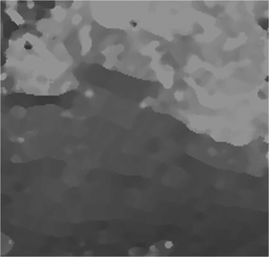
4. Co-Registration Based on Three Parts of Two Complex Images and Contoured Windows for Synthetic Aperture Radar Interferometry

In the InSAR data processing, the precise registration technique of the two single look complex images is one of the key factors in improving the measurement accuracy. The registration error is one main source of the noises in the interferometric phase image. The improvement of the registration accuracy and reduction of registration error is of great significance in improving the quality of the interferometric phase image, reducing the difficulty of phase unwrapping, and improving the unwrapping precision.

With the illumination of the above CCI method to generate InSAR phase images, we propose the new InSAR registration criterion based on the correlation coefficient of three parts, according to which only any three parts of the complex images are needed, and the registration result is better than that using the conventional relevant coefficient registration criterion.

The formula induction of the new registration criterion $g$ is similar to that in CCI and thus it will only be briefly introduced. As for the detailed induction, please refer to Ref. 10. The correlation formulae used can be such mathematic expression as standardized correlation, standardized covariance correlation, etc. Here we take the standardized correlation as an example to illustrate the induction:

Eq. (27)

C (r, x) = \frac{{〈 f_{1} \cdot f_{2} 〉}_{m \times n}}{\sqrt{{〈 f_{1}^{2} 〉}_{m \times n} \cdot {〈 f_{2}^{2} 〉}_{m \times n}}} .

First mutually correlate the real part of the master image with that of the slave image and calculate their self-correlation coefficient, so we have

Eq. (28)

{〈 a_{1} a_{2} 〉}_{m \times n} = {〈 A_{1} \cos (ϕ_{1 c} + u_{1}) \cdot A_{2} \cos (ϕ_{2 c} + u_{2}) 〉}_{m \times n} = {〈 \frac{1}{2} A_{1} A_{2} \cdot [\cos (ϕ_{1 c} + ϕ_{2 c} + u_{1} + u_{2}) + \cos (ϕ_{1 c} - ϕ_{2 c} + u_{1} - u_{2})] 〉}_{m \times n} .

Eq. (29)

{〈 a_{1} a_{2} 〉}_{m \times n} = {〈 A_{1} \cos (ϕ_{1 c} + u_{1}) \cdot A_{2} \cos (ϕ_{2 c} + u_{2}) 〉}_{m \times n} = {〈 \frac{1}{2} A_{1} A_{2} \cdot [\cos (ϕ_{1 c} + ϕ_{2 c} + u_{1} + u_{2}) + \cos (ϕ_{1 c} - ϕ_{2 c} + u_{1} - u_{2})] 〉}_{m \times n} = \frac{1}{2} {〈 A_{1} A_{2} 〉}_{m \times n} \cdot {〈 1 + \cos (2 ϕ_{1 c} + 2 u_{1}) 〉}_{m \times n}

Eq. (30)

{〈 a_{1} a_{2} 〉}_{m \times n} = \frac{1}{2} {〈 A_{1} A_{2} 〉}_{m \times n} \cdot {〈 1 + \cos (2 ϕ_{2 c} + 2 u_{2}) 〉}_{m \times n},

based on which we have

Eq. (31)

C_{1} = \frac{{〈 A_{1} A_{2} 〉}_{m \times n} \cdot {〈 \cos (ϕ_{1 c} + ϕ_{2 c} + u_{1} + u_{2}) + \cos (ϕ_{1 c} + ϕ_{2 c} + u_{1} - u_{2}) 〉}_{m \times n}}{\sqrt{{〈 A_{1}^{2} 〉}_{m \times n} \cdot {〈 1 + \cos (2 ϕ_{1 c} + 2 u_{1}) 〉}_{m \times n} \cdot {〈 A_{2}^{2} 〉}_{m \times n} \cdot {〈 1 + \cos (2 ϕ_{2 c} + 2 u_{2}) 〉}_{m \times n}}} = \frac{{〈 A_{1} A_{2} 〉}_{m \times n}}{\sqrt{{〈 A_{1}^{2} 〉}_{m \times n} \cdot {〈 A_{2}^{2} 〉}_{m \times n}}} \cdot {〈 \cos (Δ ϕ_{c} + Δ u) 〉}_{m \times n} .

Similarly, put the real part of the master image and the imaginary part of the slave part into Eq. (27), and we have

C_{2}

.

Based on $C_{1}$ and $C_{2}$ , we define the following registration criterion:

Eq. (32)

g = \sqrt{C_{1}^{2} + C_{2}^{2}} = \frac{| {〈 A_{1} A_{2} 〉}_{m \times n} |}{\sqrt{{〈 A_{1}^{2} 〉}_{m \times n} \cdot {〈 A_{2}^{2} 〉}_{m \times n}}} \cdot \sqrt{{〈 \cos (Δ ϕ_{c} + Δ u 〉}_{m \times n}^{2} + {〈 \sin (Δ ϕ_{c} + Δ u 〉}_{m \times n}^{2}} .

To improve the registration accuracy and reduce the impact of the phase gradient on the correlation, we further propose to do the above correlation calculation in the phase-contoured window. As illustrated previously, the difference

Δ u

between

u_{1}

and

u_{2}

is small, around zero, and zero being its mean value. Suppose the window is large enough, we can get Eq. (14).

$Δ ϕ_{c}$ is a constant within the contoured window. Put it into Eq. (32) and we have

Eq. (33)

{〈 \cos (Δ ϕ_{c} + Δ u) 〉}_{m \times n} = {〈 \cos Δ ϕ_{c} \cos Δ u - \sin Δ ϕ_{c} \sin Δ u 〉}_{m \times n} = \cos Δ ϕ_{c} {〈 \cos Δ u 〉}_{m \times n}

Eq. (34)

{〈 \sin (Δ ϕ_{c} + Δ u) 〉}_{m \times n} = {〈 \sin Δ ϕ_{c} \cos Δ u - \cos Δ ϕ_{c} \sin Δ u 〉}_{m \times n} = \sin Δ ϕ_{c} {〈 \cos Δ u 〉}_{m \times n} .

Put Eqs. (33) and (34) into Eq. (32), we have

Eq. (35)

g = \sqrt{C_{1}^{2} + C_{2}^{2}} = \frac{| {〈 A_{1} A_{2} 〉}_{m \times n} |}{| {〈 A_{1}^{2} 〉}_{m \times n} \cdot {〈 A_{2}^{2} 〉}_{m \times n} |} \cdot {〈 \cos Δ u 〉}_{m \times n} .

From Eq. (35) we directly get the relationship between

g

and

Δ u

, which shows that when the two complex images registered completely, the decorrelation noise

Δ u

should be the smallest. The smaller

Δ u

is, the larger

g

is, the better the corresponding registration is, which is in accordance with the physical concept. Compared with Eq. (32), Eq. (35) is free of the influence of

Δ ϕ_{c}

with the physical significance clearer.

Figure 6 is the flowchart of the three parts registration method.

Fig. 6

The flowchart of the three parts registration method.

5. Experimental Results of CCI in InSAR Data Processing

To prove the effectiveness of CCI proposed in this paper, we would like to use CCI to process real InSAR data, which are from ERS1/2. Figure 7 is the result comparison of three parts registration method and the four parts correlation coefficient registration method. Compared in the figure are the correlation coefficients of the corresponding master image and the slave image after they have been registered with the two methods. The $x$ -axis is the correlation coefficient, and the $y$ -axis is the number of pixels. The figure shows that the correlation coefficients with the method proposed in this paper are all higher than those with the conventional method. This means that the method proposed in this paper is more accurate, though only three parts are used.

Fig. 7

The correlation comparison between our registration method and traditional registration method based on correlation coefficient.

Figure 8(a) is the interferometric phase image generated with the conventional complex conjugate multiplicative method after the registration with three parts registration method; Fig. 8(b) is the phase image generated with CCI. Figure 8 shows that the three parts registration method is right and effective, and the phase image generated with CCI three parts is obviously better than that generated with the conventional four parts. With CCI, we can get the smooth phase image with almost no phase noises, while also the fringe phase is well kept without the blurring effect.

Fig. 8

Image (a) is obtained with complex conjugate multiplicative method after registered by our three image method; image (b) is obtained by our CCI method.

As illustrated previously, in the CCI formula induction, we can choose direct correlation, standardized correlation, and standardized covariance correlation, etc. The original data in Fig. 9 is the same as that in Fig. 8. Figure 9(a) is the interferometric phase image generated by calculation of each pixel (the window is $1 \times 1$ ) with the covariance correlation formula CCI method, which is different from the direct correlation formula induced in this paper. From the figure, we can see that the phase can’t be obtained by the covariance correlation formula. Figure 9(b) is the result of direct correlation method proposed in this paper. Since we, in fact, did not do the correlative average calculation, the conditions of Eqs. (11) and (12) are not satisfied. Therefore, the original phase $ϕ_{1 c}$ , $ϕ_{2 c}$ , and the random noises $u_{1}$ and $u_{2}$ are all preserved in the generated image. The noise is larger than the decorrelation noise with the conventional complex conjugate multiplicative method.

Fig. 9

Phase images obtained with rectangle windows by CCI method. Image (a) is by the covariance correlation method with windows of $1 \times 1$ ; (b) is by direct correlation with windows of $1 \times 1$ . Images (c) and (d) are obtained by the covariance correlation method with $5 \times 5$ windows and $9 \times 9$ windows, respectively.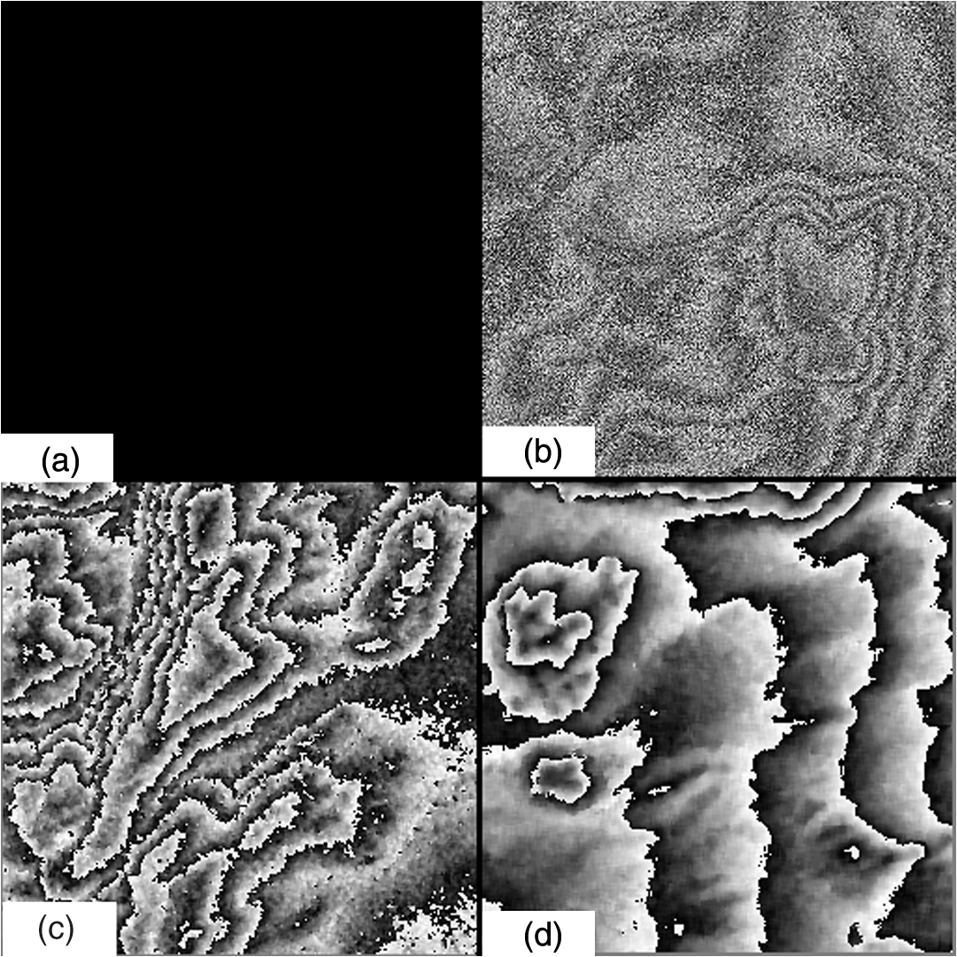

Figure 9(c) and 9(d) are the interferometric phase images generated with the covariance correlation formula CCI method after being correlated in the rectangular windows $5 \times 5$ and $9 \times 9$ , respectively. With the window increasing, the random phase noises decreases quickly. Figure 9 shows that after the correlation calculation in a window of certain size, the phase noises will be quickly removed, for the phase noises conform to the statistical rules in Eqs. (11), (12), and (14). Figure 9 also shows that the result is worse when the covariance correlation formula CCI method with which the mean value is deducted is adopted in a small window, compared with the CCI method proposed in this paper. Accordingly, the proposed direct correlation formula should be adopted.

The comparison also shows that we can obtain a better phase image with the rectangular window three parts generation method, but it is worse than that generated with the contoured window, for it has some blurring effect. Although only an approximate fringe pattern is generated with the rectangular window, this is one of the important steps in the three parts registration and the interferometric phase image generation, for it provides the fringe orientation with the three parts, making the need of the method for the three parts a closed loop and the method perfect. Without such a step, the fringe orientation would be obtained only through the fringe pattern generated with the conventional complex conjugate multiplicative method and thus the four parts would have to be used, but not the three parts in the last stage.

Figure 10 is the result comparison of the real airborne InSAR data processing with CCI and the conventional complex conjugate multiplicative method. Due to the small decorrelation noise with the airborne InSAR data, the complex conjugate multiplicative method can also arrive at a good result. But the noise in the phase image generated with CCI is smaller. Figure 11 is the result comparison of the CCI processing of different real and imaginary parts of the two complex images in different areas with the same set of data. Take any three parts from the four parts ( $a_{1}$ , $a_{2}$ , $b_{1}$ , $b_{2}$ ), and we have four different combinations ( $a_{1}$ , $b_{1}$ , $a_{2}$ ), ( $a_{1}$ , $b_{2}$ , $a_{2}$ ), ( $b_{1}$ , $a_{1}$ , $b_{2}$ ), and ( $b_{1}$ , $a_{2}$ , $b_{2}$ ). From the image, we can see that the processing results of the four sets with CCI are almost the same, proving that the selection of parts with CCI is arbitrary.

Fig. 10

The comparison between our method (right) and traditional method (left) for airborne InSAR data.

Fig. 11

Four results of our method with different choices of part images.

Figure 12 is the processing result of the same area with serious decorrelation noise with the conventional complex conjugate multiplicative method (left half) and CCI (right half). It shows that for the area with lower correlation, it is difficult to process by the conventional method, but CCI can still result in good phase message. The theoretical analysis and many experimental results show that as long as the approximately right fringe-orientation map (namely, the fringe-contoured window), is obtained, we can to a great extent reduce or even remove the decorrelation effect by doing the correlation calculation with CCI on the approximate contour. For the area with serious decorrelation, we can still obtain the phase undisturbed and the phase noises removed.

Fig. 12

The comparison between our method (right) and traditional method (left) for a poor quality InSAR data.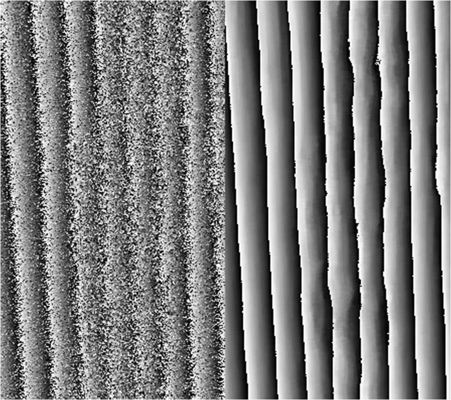

Figure 13(a) and 13(b) are the results of InSAR data over Mount Etna volcano in Italy whose fringe pattern is with fast variations. Figures 12 and 13 show that CCI can still result in a good phase message in the area with poor correlation, which is difficult to process by the conventional method. Both theoretical analysis and many experimental results show that as long as the approximately right fringe-orientation map (namely, the fringe-contoured window) is obtained, we can to a great extent reduce or even remove the decorrelation effect by doing the correlation calculation with CCI on the approximate contoured windows. For the area with serious decorrelation, we can still obtain the undisturbed phase with the phase noises being removed.

Fig. 13

Comparison of the results got from traditional CCMM method (a) and our CCI method (b) for poor quality InSAR data (Over Mount Etna volcano in Italy).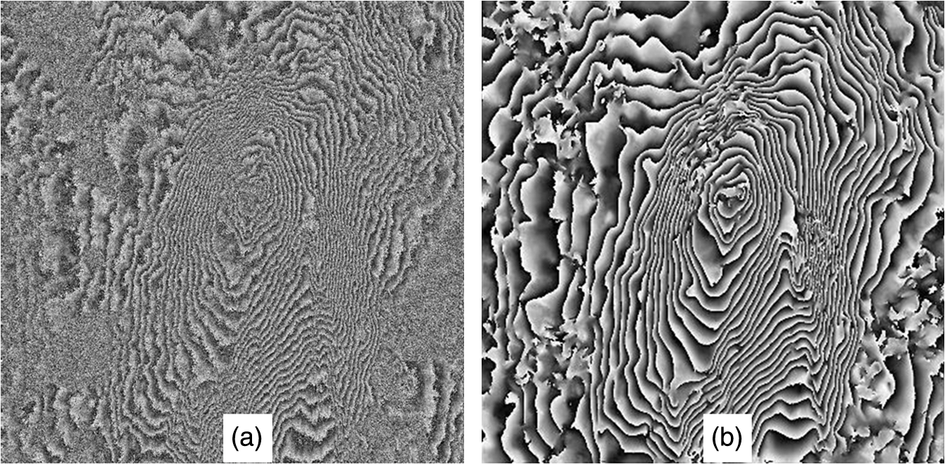

Due to the slower change of the fringe orientation than the phase (namely, the fringe), the recovery of the approximate fringe orientation is much easier and more reliable than that of the right phase, especially for the area with obvious decorrelation. Therefore CCI can effectively improve the adaptation and the applicability of the InSAR data. Besides, the experiment shows that CCI is not quite sensitive to the precision of the contoured window; the contoured window with some error still being able to get better results than the conventional rectangular window.

6. Conclusion

In this paper, the proposed registration method and phase image-generation method based on three parts of the InSAR complex image pair are systematically illustrated and expanded. The adaptation and the precision of CCI method, the improved key steps, and the determination of the contoured window are also analyzed. The processing result of the real data has proved that the three parts registration method is more accurate than the conventional correlation coefficient-based registration method and is a brand-new concept of InSAR data-processing method. The phase image with the method proposed in this paper contains almost no phase noises, preserves the fringe at the same time, and is free of the blurring effect. As for the conventional method, while the phase noises are reduced, the signal is blurred. Although CCI is more complicated than the conventional method, the generated phase image is void of the phase noises, which saves the trouble of filtering in post-processing.

What’s more important, the proposed registration method and the interferometric phase image-generation method contribute to forming a complete InSAR data-processing method that involves only three parts. For the space-borne InSAR system, if the imaging is to be completed on the satellite, only any three of the four parts need to be transmitted back to the earth to finish the InSAR data processing, greatly reducing the transmission load, which is of great significance for the transmitting and processing of the space-borne InSAR data. One of the critical steps with CCI is the obtaining of the contoured windows, for which we will do some further research concerning how to determine the contoured windows with better self-adaptation, higher efficiency, and greater precision.

Acknowledgments

This research is funded by the National Nature Science Foundation of China (Grant No. 40901215 & 11002156) and the Foundation of National University of Defense Technology.

References

1.

P. A. RosenS. HensleyI. R. Joughin, “Synthetic aperture radar interferometry,” Proc. IEEE, 88 (3), 333 –382 (2000). http://dx.doi.org/10.1109/5.838084 IEEPAD 0018-9219 Google Scholar

2.

R. BamlerP. Hartl, “Synthetic aperture radar interferometry,” Inverse Probl., 14 (4), R1 –R54 (1998). http://dx.doi.org/10.1088/0266-5611/14/4/001 INPEEY 0266-5611 Google Scholar

3.

J.-S. Leeet al., “A new technique for noise filtering of SAR interferometric phase images,” IEEE Trans. Geosci. Rem. Sens., 36 (5), 1456 –1465 (1998). http://dx.doi.org/10.1109/36.701024 IGRSD2 0196-2892 Google Scholar

4.

H. LiG. Liao, “An estimation method for InSAR interferometric phase based on MMSE criterion,” IEEE Trans. Geosci. Rem. Sens., 48 (3), 1457 –1469 (2010). http://dx.doi.org/10.1109/TGRS.2009.2031100 IGRSD2 0196-2892 Google Scholar

5.

B. YongB. Mercer, “Interferometric SAR phase filtering in the wavelet domain using simultaneous detection and estimation,” IEEE Trans. Geosci. Rem. Sens., 49 (4), 1396 –1416 (2011). http://dx.doi.org/10.1109/TGRS.2010.2076286 IGRSD2 0196-2892 Google Scholar

6.

Q. Wanget al., “An efficient and adaptive approach for noise filtering of SAR interferometric phase images,” IEEE Geosci. Rem. Sens. Lett., 8 (6), 1140 –1144 (2011). http://dx.doi.org/10.1109/LGRS.2011.2158289 IGRSBY 1545-598X Google Scholar

7.

Q. Yuet al., “Single-phase-step method with contoured correlation fringe patterns for ESPI,” Opt. Express, 12 (20), 4980 –4985 (2004). http://dx.doi.org/10.1364/OPEX.12.004980 OPEXFF 1094-4087 Google Scholar

8.

Q. Yuet al., “Co-registration based on three parts of two complex images and contoured windows for synthetic aperture radar interferometry,” IEEE Geosci. Rem. Sens. Lett., 4 (2), 288 –292 (2007). http://dx.doi.org/10.1109/LGRS.2007.894146 IGRSBY 1545-598X Google Scholar

9.

Q. YuS. FuH. Mayer, “Generation of speckle-reduced phase images from three complex parts for SAR interferometry,” Appl. Phys. Lett., 88 (11), 114106 (2006). http://dx.doi.org/10.1063/1.2185250 APPLAB 0003-6951 Google Scholar

10.

Q. Yu, “Spin filtering process and automatic extraction of fringe center-lines from interferometric patterns,” Appl. Opt., 27 (18), 3782 –3784 (1988). http://dx.doi.org/10.1364/AO.27.003782 APOPAI 0003-6935 Google Scholar

11.

Q. YuX. SunX. Liu, “Spin filtering with curve windows for interferometric fringes,” Appl. Opt., 41 (14), 2650 –2654 (2002). http://dx.doi.org/10.1364/AO.41.002650 APOPAI 0003-6935 Google Scholar

12.

Q. Yuet al., “An adaptive contoured window filter for interferometric synthetic aperture radar,” IEEE Geosci. Rem. Sens. Lett., 4 (1), 23 –26 (2007). http://dx.doi.org/10.1109/LGRS.2006.883527 IGRSBY 1545-598X Google Scholar

13.

M. KassA. Witkin, “Analyzing oriented patterns,” Comp. Vis. Graph. Image Proc., 37 (3), 362 –385 http://dx.doi.org/10.1016/0734-189X(87)90043-0 CVGPDB 0734-189X Google Scholar

14.

S. Fuet al., “Directionally adaptive filter for synthetic aperture radar interferometric phase images,” IEEE Trans. Geosci. Rem. Sens., 51 (1), 552 –559 (2012). http://dx.doi.org/10.1109/TGRS.2012.2202911 IGRSD2 0196-2892 Google Scholar

15.

R. BamlerP. Hartl, “Synthetic aperture radar interferometry,” Inverse Probl., 14 (4), R1 –R54 (1998). http://dx.doi.org/10.1088/0266-5611/14/4/001 INPEEY 0266-5611 Google Scholar

16.

J. W. Goodman, Laser Speckle and Related Phenomena, Springer-Verlag, Berlin (1975). Google Scholar

Biography

Jianhua Shi is an associate professor at the National University of Defense Technology in China. She received her PhD degrees in optical engineering from the National University of Defense Technology in 2004. She is the author of about 20 journal papers and has written two book chapters. Her current research interests include interferogram processing and applied laser technology.

Sihua Fu received his BS, MS, and PhD degrees in aeronautical and astronautical science and technology from the National University of Defense Technology, P. R. China, in 1999, 2002, and 2006, respectively. He was with the National University of Defense Technology as an assistant professor in 2006. From 2010, he is an associate professor with the College of Opto-Electronic Science and Engineering. His research topics include image measurement technologies, InSAR data processing and optical interferometic fringes processing.

CC BY: © The Authors. Published by SPIE under a Creative Commons Attribution 4.0 Unported License. Distribution or reproduction of this work in whole or in part requires full attribution of the original publication, including its DOI.

Citation Download Citation

Jianhua Shi, Sihua Fu, Xuejun Long, Xia Yang, and Qifeng Yu "Contoured window correlation interferometry for synthetic aperture radar interferometry based on three parts of complex images," Journal of Applied Remote Sensing 7(1), 073559 (22 May 2013). https://doi.org/10.1117/1.JRS.7.073559

Published: 22 May 2013

Access the abstract

JOURNAL ARTICLE
18 PAGES

DOWNLOAD PAPER SAVE TO MY LIBRARY

GET CITATION

KEYWORDS

Interferometry

Interferometric synthetic aperture radar

Phase interferometry

Image registration

Synthetic aperture radar

Data processing

Fringe analysis

1.

Introduction

2.

Defining of the Contoured Window of the InSAR Phase Image

2.1.

Calculation of Fringe Orientation Map

Eq. (1)

Eq. (2)

Eq. (3)

Eq. (4)

Fig. 1

Fig. 2

2.2.

Determination of the Fringe Contoured Window

Eq. (5)

Fig. 3

2.3.

Determination of the Size of Fringe-Contoured Window

Fig. 4

Fig. 5

3.

Contoured Correlation Interferometry to Generate InSAR Phase Images

3.1.

Current Complex Conjugate Multiplicative Method

Eq. (6)

Eq. (7)

Eq. (8)

3.2.

CCI Formulae Induction

Eq. (9)

Eq. (10)

Eq. (11)

Eq. (12)

Eq. (13)

Eq. (14)

Eq. (15)

Eq. (16)

Eq. (17)

Eq. (18)

Eq. (19)

3.3.

Formulae Induction of the Correlation Interferometry with Rectangular Window

Eq. (20)

Eq. (21)

Eq. (22)

Eq. (23)

Eq. (24)

Eq. (25)

Eq. (26)

3.4.

Principle Steps to Generate InSAR Interferometric Phase Image with CCI Method

4.

Co-Registration Based on Three Parts of Two Complex Images and Contoured Windows for Synthetic Aperture Radar Interferometry

Eq. (27)

Eq. (28)

Eq. (29)

Eq. (30)

Eq. (31)

Eq. (32)

Eq. (33)

Eq. (34)

Eq. (35)

Fig. 6

5.

Experimental Results of CCI in InSAR Data Processing

Fig. 7

Fig. 8

Fig. 9

Fig. 10

Fig. 11

Fig. 12

Fig. 13

6.

Conclusion

Acknowledgments

References

Biography

Show All Keywords

Keywords/Phrases

Search In: