|
|
1.IntroductionCoastal waters occupy at the most 8–10% of the ocean surface and only 0.5% of its volume, but represent an important fraction in terms of economic, social, and ecological value.1 Coastal waters are also under the greatest anthropogenic pressure. As a result, there is strong need to monitor coastal environments. By monitoring changes in water quality we can observe, assess, and correct long term trends in water quality degradation. It is obvious that the infrequent measurements from research vessels or automated measuring systems on ships of opportunity or buoys cannot provide the spatial and temporal coverage needed for monitoring such dynamic environments like coastal waters.2 Remote sensing can provide greater spatial coverage with finer spatial resolution and often with good temporal frequency. This makes remote sensing a rich source of data.3 The remote sensing signal is determined by the amount of optically active substances like phytoplankton (usually measured as concentration of chlorophyll-a), suspended matter, and colored dissolved organic matter (CDOM). In optically simple oceanic waters, the latter two are well correlated with the phytoplankton as they are phytoplankton degradation products. In optically complex coastal and inland waters, commonly labelled as “Case II” waters,4 most of the CDOM and suspended matter originates from the adjacent land. As a result, the concentrations of these substances vary independently from each other and they may vary across a wide range (orders of magnitude). Therefore, the developing of reliable remote sensing algorithms for such waters is very complicated and the algorithms are often local or even seasonal. Another complicating aspect is vertical distribution of the optically active substances. For example, CDOM transported into marine environment by rivers may stay on the sea surface as the fresh water is lighter than the salt water.5 These effects are limited to very near coastal zone. On the other hand vertical distribution of phytoplankton may have quite significant impact on remote sensing signal over large areas. Others have shown that the vertical distribution of phytoplankton and the deep chlorophyll maximum in oceanic waters has an impact on the remotely sensed signal.6,7 In turbid coastal waters, the depth of penetration of light (the depth where remote sensing signal is formed) is often relatively shallow (a few meters to centimeters). On the other hand Kutser et al.8 have shown that vertical distribution of phytoplankton may have significant impact on the remote sensing signal. Especially in the case of cyanobacteria that can regulate their buoyancy and migrate in water column to the depth optimal for their growth. There is little information available about the vertical distribution of chlorophyll-a in the southern Caspian Sea. In the southern Caspian Sea the thermocline starts to form in spring, sharpens in summer, begins to degrade and then completely degrades in autumn. It is usually not observed at all in winter.9 The formation and destruction of seasonal thermocline affects the chlorophyll-a concentration. The aim of our study was to measure the vertical distribution of phytoplankton (chlorophyll-a) in the southern Caspian Sea during the period when the thermocline is formed and to evaluate whether the vertical distribution of phytoplankton has an impact on the remote sensing signal complicating development of the chlorophyll-a retrieval algorithms for the coastal waters of the Caspian Sea. 2.Methods2.1.Field MeasurementsField sampling was conducted in the southern Caspian Sea waters crossing a full freshwater-marine water gradient (Fig. 1). Twenty-three cruises were conducted in thirty stations during spring-summer period of 2011. The vertical profile of chlorophyll-a was measured using a seapoint chlorophyll fluorometer (SCF) that was interfaced with an Idronaut OCEAN SEVEN 316 CTD multiparameter probe. SCF is a high-performance, low power instrument for in situ measurements of chlorophyll-a. Also, the vertical profile of water turbidity was measured using an optical probe (Seapoint Turbidity Meter). This instrument measures light scattered by particles suspended in water generating an output voltage proportional to turbidity or the amount of suspended solids. The results are expressed in Formazine Turbidity Units (FTU), which may be directly related to the suspended sediment concentration.10 Fig. 1Sampling stations in the southern Caspian Sea. (There are five stations in two transects, the stations are named according to L1, L2, L3, L4, L5, A1, A2, A3, A4, A5. The distance between stations is 3 km and between two transects is 10 km).  The amount of total suspended solids, TSS, was measured by filtering 1 L water samples through preweighed 47 mm Millipore GN filters (0.45 μm pore size). Filters were dried in a desiccator and weighed again. The difference of filter weights before and after filtering the water sample, together with the volume of filtered seawater, was used to calculate the TSS concentration.11 For CDOM, seawater was filtered the same day after returning to laboratory (Central Laboratory, Faculty of Natural Resources, Tarbiat Modares University) through polycarbonate track etch membrane filters (PCMembran, 0.2 μm, 47 mm) (Sartorius-stedium). CDOM absorbance was determined between 200 nm and 850 nm using a Perkin Elmer Lambda 25 spectrophotometer in a 10 cm quartz cuvette. The Milli-Q water was used as reference and a baseline correction was applied to the data by subtracting the average between 683 nm and 687 nm to the entire spectrum.12,13 The absorbance values at each wavelength were transformed into absorption coefficients using where l is the cuvette path length (0.1 m).Absorption data were fitted with an exponential function using nonlinear regression between 350 nm and 500 nm12–14 to retrieve , the CDOM absorption estimate at a reference wavelength (375 nm) and S, the slope of the absorption curve: The absorption value at 375 nm, , was chosen to quantify CDOM.13–15 2.2.Optical ModellingThe HydroLight 5.0 radiative transfer code16 was used to simulate the remote sensing reflectance spectra. The HydroLight radiative transfer numerical model computes radiance distributions and related quantities. Users can specify the water absorption and scattering properties, the sky conditions, and the bottom boundary conditions. HydroLight then solves the scalar radiative transfer equation (RTE) to compute the in-water radiance as a function of depth, direction, and wavelength. Other quantities of interest, such as the water-leaving radiance and remote-sensing reflectance, are also obtained from the computed radiances. Caspian Sea waters belong to optically more complex Case II waters where the concentrations of optically active substances vary independently of chlorophyll-a. A Case II water model with three optically active substances (chlorophyll-a, CDOM and mineral particles) was parameterized for the Caspian Sea study in HydroLight. The mass-specific absorption and scattering coefficients of optically active substances available in the HydroLight were used as there is no information about those parameters in the Caspian Sea. The modelling was carried out over the wavelength range of 350-850 nm with 5 nm intervals. Wind speed was taken to be . The solar zenith angle was assumed to be 30 deg, which is typical for the time around midday in the July-August period when the thermocline occurs in the Caspian Sea. Eleven measuring stations were selected for the modelling study in order to describe the whole range of variability in vertical distribution of biomass as it was observed during our field campaigns. Two different HydroLight runs were made for each of the selected stations. First we used a measured chlorophyll profile (Figs. 2, 3, and 4) for each station. A second model run for each station was carried out using a constant chlorophyll-a value for the whole water column. An average chlorophyll-a of the top first meter was used for the whole water column. 3.Results and DiscussionTable 1 shows the results of field measurements of optically active constituents in three cruises. As expected, of nearer stations to the coast show much higher values compared to far stations in each cruise, i.e., and respectively. TSS concentration ranged from in near stations to coast to in the far stations from the coast. Chlorophyll showed variations, too. Near stations to the coast show much higher values compared to far stations in each cruise, i.e., and respectively (Table 1). Table 1The results of field measurements of optically active constituents.
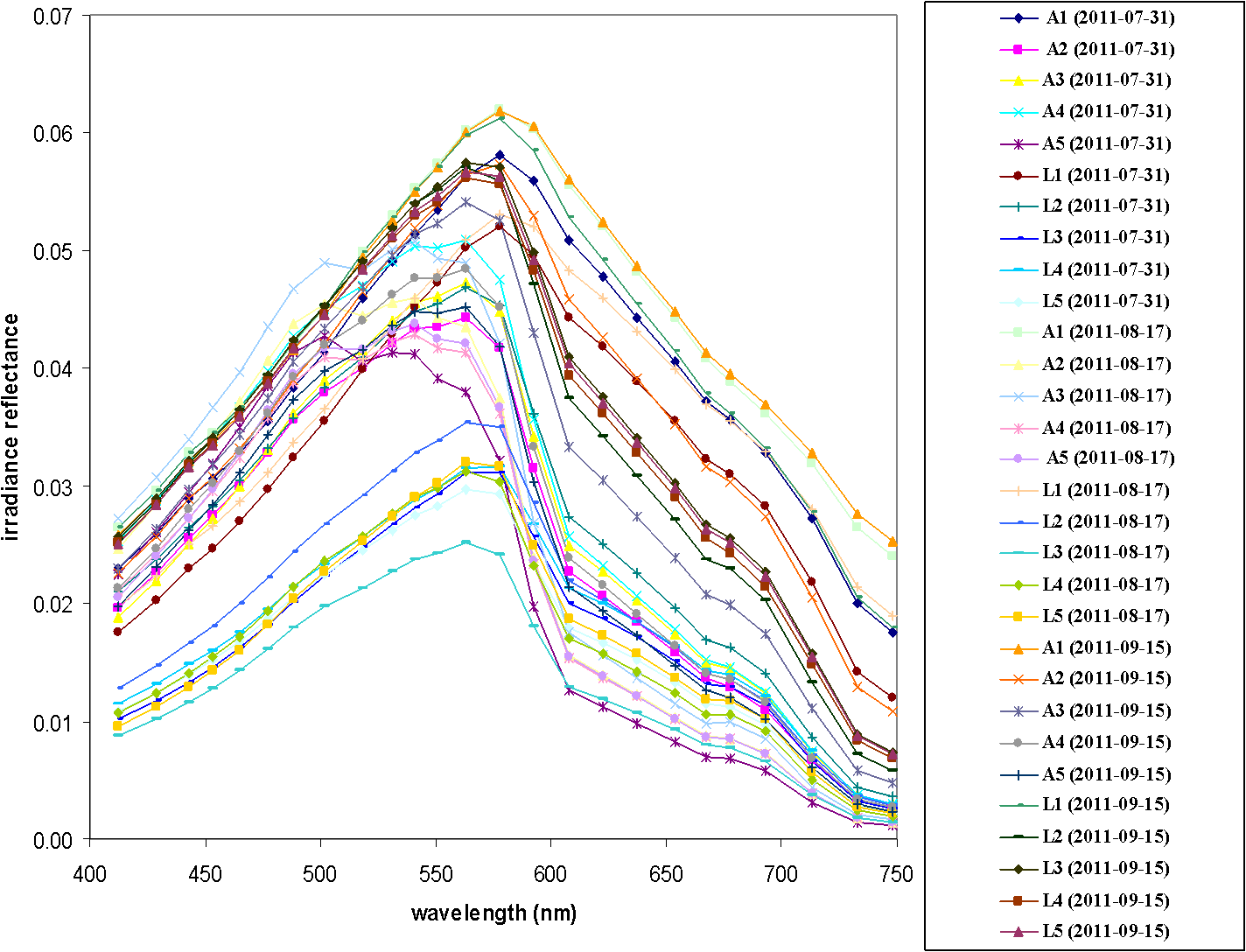
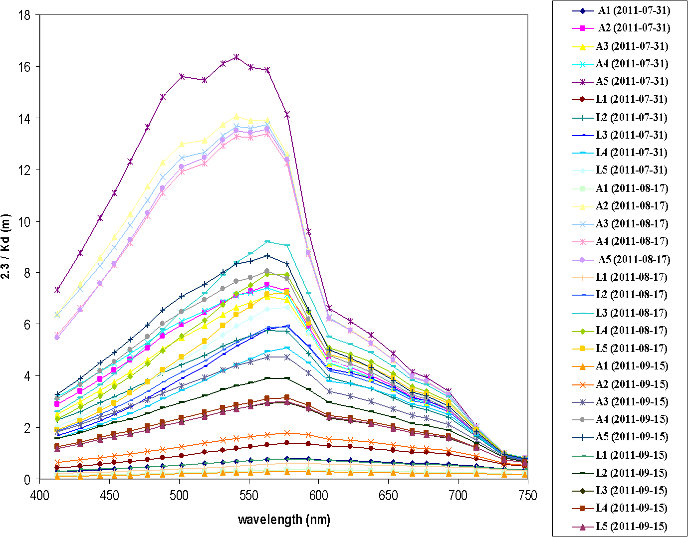
Figures 5Fig. 6Fig. 7Fig. 8Fig. 9 to 10 provide some more detailed insight into formation of the reflectance spectra revealed by the model simulations. Figures 5 and 6 show the total absorption coefficient and its components and total absorption coefficients just beneath the sea surface for two stations (A1 near to the coast, A5 far from the coast), and Figures 7 and 8 show the corresponding scattering coefficient and its components for July 2011. The total absorption is dominated by mineral particles in near stations to the coast and by the water itself in stations far from the coast. The primary scatters are mineral particles in near stations to the coast and chlorophyll-a in stations far from the coast, too. However, the water makes only a small contribution to the total scattering. The irradiance reflectance and remote-sensing reflectance , the quantity of interest for “ocean color” remote sensing, is shown in Figs. 9 and 10. As can be seen, R values become higher as turbidity increases. In this study, we assumed that the impact of vertical distribution of phytoplankton is detectable by remote sensing instruments if the difference between the two modelled spectra is higher than the signal to noise ratio of different sensors. This kind of methodology has been used to estimate if potentially toxic cyanobacterial blooms be separated from blooms of other algae,17 if remote sensing can be used to map benthic habitats in coastal waters18 and determining what type of coral reef habitats can be separated from each other.19 Figures 11 and 12 illustrate the influence of the vertical distribution of chlorophyll-a on the remote sensing signal in two stations (A3 & A5). Using the constant chlorophyll-a value through the water column produces slightly higher reflectance values than using actually measured chlorophyll-a profiles. This indicates that the vertical distribution of phytoplankton biomass has a small impact on the reflectance spectra. However, the difference between the reflectance calculated for a homogeneous water column and the reflectance calculated for the actual stratification of biomass is so small that no remote sensing sensor can detect the difference. Fig. 11Modelled remote sensing reflectance in Station A3 using the constant chlorophyll-a value through the water column and actually measured chlorophyll-a profiles.  Fig. 12Modelled remote sensing reflectance in Station A5 using the constant chlorophyll-a value through the water column and actually measured chlorophyll-a profiles. 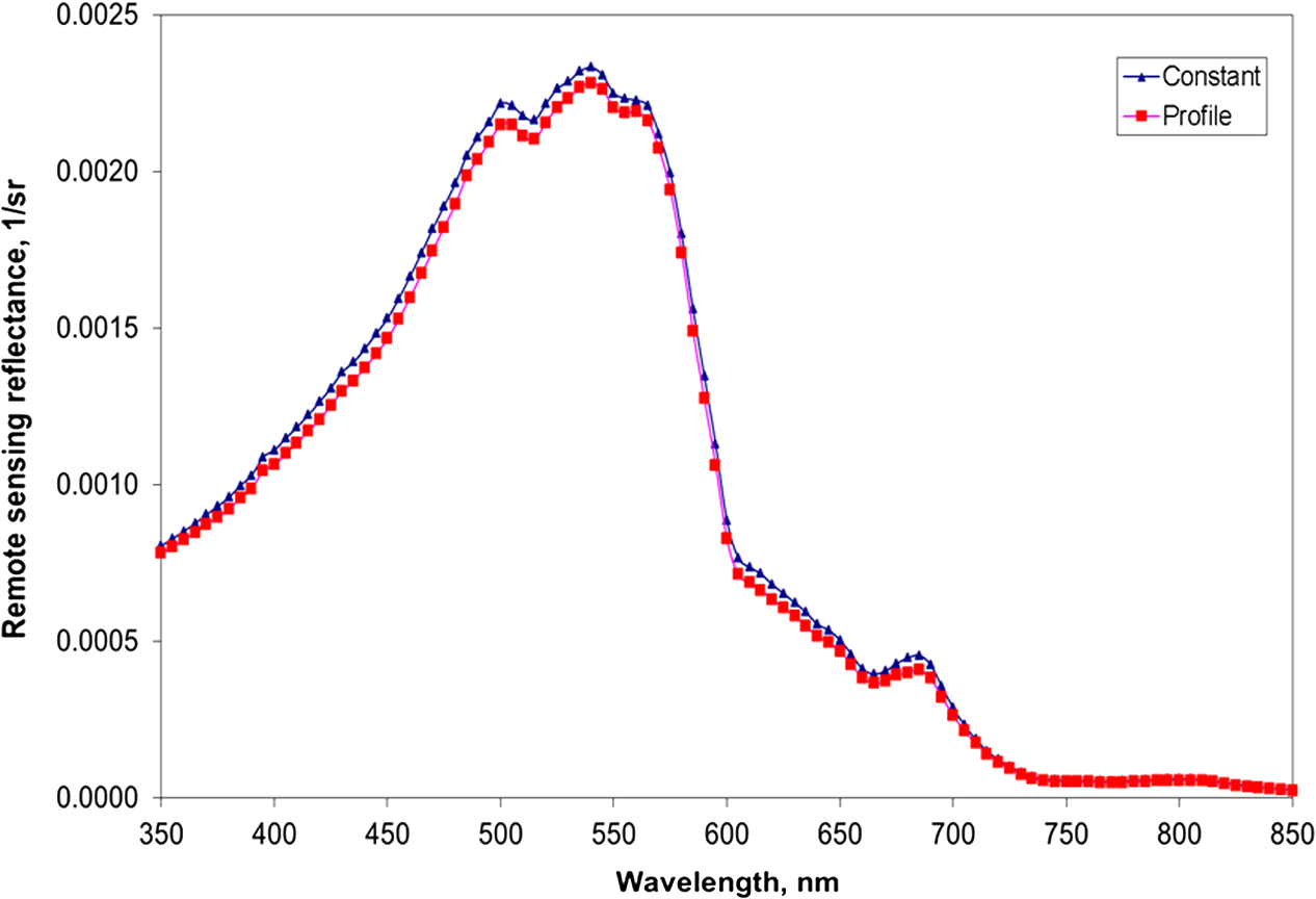 This result is not surprising if one considers that the contribution of different water layers to the total remote sensing signal decreases exponentially with increasing depth. Our estimates show that the depth of penetration (the layer from which the remote sensing signal originates) is less than 18 m (based on ) in the clearest station of study area (Fig. 13). The deep chlorophyll maximum is in deeper waters than the depth of penetration in all stations. It means that the order of magnitude increases in phytoplankton concentration cannot have impact on the remote sensing signal since the biomass peak is below the layer remote sensing sensors can “see.” The field measurements were carried out during the spring-summer period (May–September) when thermocline should occur in the southern Caspian Sea waters. During the rest of the year, the top layer of the sea is well mixed and the vertical distribution of biomass is homogenous. Therefore, our measurements should describe the range of variability in vertical distribution of phytoplankton occurring in the southern Caspian Sea. The results show that the impact of vertical distribution of phytoplankton biomass is very small in the cases where the nonuniform distributions occur. Remote sensing sensors cannot detect such a small difference. It means that taking a surface water sample for calibration and validation of remote sensing algorithms is sufficient in the southern Caspian Sea to characterize the water mass under investigation. We are planning to validate different chlorophyll-a (and other water characteristics) retrieval algorithms for the southern Caspian Sea and develop better regional algorithms if needed. The negligible impact of the deep chlorophyll maximum on the remote sensing signal suggests that only the concentrations and specific optical properties of the optically active substances (and not their vertical distribution) have to be taken into account when developing regional algorithms for retrieval of water characteristics in the southern Caspian Sea. AcknowledgmentsThe study presented here is part of the dissertation in partial fulfillment of the requirements for the degree of PhD in Tarbiat Modarres University (TMU) of Iran. The authors extend their appreciation for the support provided by the authorities of the Tarbiat Modares University in funding the study and presenting its results in JARS. First and foremost, I would like to express my sincere thanks to Mrs. Mina Emadi Shaibani for supporting and encouraging the research. I am grateful to Dr. Nemat Mahmoudi for continuing encouragement and support in the preparation of the field data. Also, thanks to Mr. Engr. Mahmoud Valizadeh and Mr. Gholizadeh for several suggestions concerning sampling affairs. We also thank the anonymous reviewers for their constructive suggestions and comments. ReferencesN. HoepffnerG. Zibordi,
“Remote sensing of coastal waters,”
Encyclopedia of Ocean Sciences, 732
–741 2nd ed.Elsevier, Amsterdam, The Netherlands
(2009). Google Scholar
T. Kutser,
“Quantitative detection of chlorophyll in cyanobacterial blooms by satellite remote sensing,”
Limnol. Oceanogr., 49
(6), 2179
–2189
(2004). http://dx.doi.org/10.4319/lo.2004.49.6.2179 LIOCAH 0024-3590 Google Scholar
P. Biermanet al.,
“A review of methods for analysing spatial and temporal patterns in coastal water quality,”
Ecol. Indicat., 11
(1), 103
–114
(2011). http://dx.doi.org/10.1016/j.ecolind.2009.11.001 EICNBG 1470-160X Google Scholar
A. MorelL. Prieur,
“Analysis of variations in ocean color,”
Limnogy Oceanogr., 22
(4), 709
–722
(1977). http://dx.doi.org/10.4319/lo.1977.22.4.0709 LIOCAH 0024-3590 Google Scholar
L. A. Clementsonet al.,
“Properties of light absorption in a highly coloured estuarine system in south-east Australia which is prone to blooms of the toxic dinoflagellate Gymnodinium catenatum,”
Estuar. Coast. Shelf Sci., 60
(1), 101
–112
(2004). http://dx.doi.org/10.1016/j.ecss.2003.11.022 ECSSD3 0272-7714 Google Scholar
H. R. GordonD. K. Clark,
“Remote sensing optical properties of a stratified ocean: an improved interpretation,”
Appl. Opt., 19
(20), 598
–600
(1980). http://dx.doi.org/10.1364/AO.19.000598 APOPAI 0003-6935 Google Scholar
M. StramskaD. Stramski,
“Effects of non-uniform vertical profile of chlorophyll concentration on remote-sensing reflectance of the ocean,”
Appl. Opt., 44 1735
–1747
(2005). http://dx.doi.org/10.1364/AO.44.001735 APOPAI 0003-6935 Google Scholar
T. L. KutserL. MetsamaaA. G. Dekker,
“Influence of the vertical distribution of cyanobacteria in the water column on the remote sensing signal,”
Estuar. Coast. Shelf Sci., 78
(4), 649
–654
(2008). http://dx.doi.org/10.1016/j.ecss.2008.02.024 ECSSD3 0272-7714 Google Scholar
A. Roohiet al.,
“Changes in biodiversity of phytoplankton, zooplankton, fishes and macrobenthos in the Southern Caspian Sea after the invasion of the ctenophore Mnemiopsis Leidyi,”
Biol. Invas., 12
(7), 2343
–2361
(2010). http://dx.doi.org/10.1007/s10530-009-9648-4 1387-3547 Google Scholar
V. VolpeS. SilvestriM. Marani,
“Remote sensing retrieval of suspended sediment concentration in shallow waters,”
Rem. Sens. Environ., 115
(1), 44
–54
(2011). http://dx.doi.org/10.1016/j.rse.2010.07.013 RSEEA7 0034-4257 Google Scholar
J. L. Muelleret al.,
“Ocean optics protocols for satellite ocean color sensor validation: biogeochemical and bio-optical measurements and data analysis protocols,”
(2003). Google Scholar
M. Babinet al.,
“Variations in the light absorption coefficients of phytoplankton, nonalgal particles, and dissolved organic matter in coastal waters around Europe,”
J. Geophys. Res., 108
(C7), 3211
(2003). http://dx.doi.org/10.1029/2001JC000882 JGREA2 0148-0227 Google Scholar
R. AstorecaV. RousseauC. Lancelot,
“Coloured dissolved organic matter (CDOM) in Southern North Sea waters: Optical characterization and possible origin,”
Estuar. Coast. Shelf Sci., 85
(4), 633
–640
(2009). http://dx.doi.org/10.1016/j.ecss.2009.10.010 ECSSD3 0272-7714 Google Scholar
A. BricaudA. MorelL. Prieur,
“Absorption by dissolved organic matter of the sea (yellow substance) in the UV and visible domains,”
Limnol. Oceanogr., 26
(1), 43
–53
(1981). http://dx.doi.org/10.4319/lo.1981.26.1.0043 LIOCAH 0024-3590 Google Scholar
C. A. StedmonS. Markager,
“The optics of chromophoric dissolved organic matter (CDOM) in the Greenland Sea: an algorithm for differentiation between marine and terrestrially derived organic matter,”
Limnol. Oceanogr., 46
(8), 2087
–2093
(2001). http://dx.doi.org/10.4319/lo.2001.46.8.2087 LIOCAH 0024-3590 Google Scholar
C. D. MobleyL. K. Sundman, Hydrolight 5 Users’ Guide, Sequoia Scientific, Inc., Redmond, WA
(2008). Google Scholar
L. MetsamaaT. KutserN. Strömbeck,
“Recognising cyanobacterial blooms based on their optical signature: a modelling study,”
Boreal Environ. Res., 11
()), 493
–506
(2006). BEREF7 1239-6095 Google Scholar
E. Vahtmäeet al.,
“Feasibility of hyperspectral remote sensing for mapping benthic macroalgal cover in turbid coastal waters,”
Rem. Sens. Environ., 101
(3), 342
–351
(2006). http://dx.doi.org/10.1016/j.rse.2006.01.009 RSEEA7 0034-4257 Google Scholar
T. KutserA. G. DekkerW. Skirving,
“Modelling spectral discrimination of Great Barrier Reef benthic communities by remote sensing instruments,”
Limnol. Oceanogr., 48
(1, part2), 497
–510
(2003). http://dx.doi.org/10.4319/lo.2003.48.1_part_2.0497 LIOCAH 0024-3590 Google Scholar
Biography Mehdi Gholamalifard is currently a PhD student of environmental pollutions (satellite monitoring) at the Tarbiat Modares University (TMU) in Iran. He received his MSc in environment from TMU, Iran, in 2006 based on his applied research on spatial-temporal modeling of MSW landfill supply and demand using SLEUTH urban growth model (UGM) in a GIS environment. He finished his BSc on environment at IAU-Arak in 22th July 2004. He received full scholarship from the Ministry of Science, Research and Technology to obtain a PhD degree at TMU. Also, he received the Erasmus Mundus research fellowship at the Faculty of Geo-Information Science and Earth Observation (ITC), The Netherlands, in Autumn 2012. His research interest focuses on environmental assessment and modeling, satellite monitoring, and geoinformatics applications in decision making. |