1.

Introduction

Technological advances in imaging spectrometry have led to acquisition of data that exhibit extremely high spatial, spectral, and radiometric resolution. As an example, a challenge of satellite hyperspectral imaging is data compression for dissemination to users and especially for transmission to a ground station from the orbiting platform. Data compression generally performs a decorrelation of the correlated information source, before entropy coding is carried out. To meet the quality issues of hyperspectral image analysis, differential pulse code modulation (DPCM) is usually employed for lossless/near-lossless compression, i.e., the decompressed data have a user-defined maximum absolute error, which is zero in the lossless case and nonzero otherwise.¹ DPCM basically consists of a prediction followed by entropy coding of quantized differences between original and predicted values. A unity quantization step size allows reversible compression as a limit case. Several variants exist in DPCM prediction schemes, the most sophisticated being adaptive.^2–8

When the hyperspectral imaging instrument is placed on a satellite, data compression is crucial.^9–11 To meet the quality issues of hyperspectral imaging, DPCM is usually employed for either lossless or near-lossless compression. Lossless compression thoroughly preserves the information of the data but allows a moderate decrement in transmission rate to be achieved.^12,13 The bottleneck of downlink to ground stations may hamper the coverage capabilities of modern satellite instruments. If strictly lossless techniques are not used, a certain amount of information of the data will be lost. However, such statistical information may be mostly due to random fluctuations of the instrumental noise. The rationale that compression-induced distortion may be less harmful in those bands, in which the noise is higher, constitutes the virtually lossless paradigm,¹⁴ which is accepted by several authors,¹⁵ but has never been demonstrated.

This paper faces the problem of quantifying the trade-off between compression ratio (CR) and decrement in the spectral information content. A rate distortion model is used to quantify the compression of the noisy version of an ideal information source. The rationale of such a model is that lossy/near-lossless compression may be regarded as an additional source of noise. The problem of lossy compression becomes a transcoding problem (cascade of two coding stages interleaved by a decoding stage), which can be formulated as “Given a source that has been compressed with loss and decompressed, and hence it has already lost part of its information, what is the relationship between the compression ratio, or bit rate (BR), of the subsequent compression stage and the amount of the information of the original source that is available from the decompressed bit stream?”

Fig. 1

Flow chart of satellite hyperspectral processing chain comprising satellite segment, ground segment, and user segment. Data are compressed to pass from one segment to another and decompressed before the subsequent processing.

Starting from the observation that the onboard instrument introduces noise on the noise-free spectral radiance that is acquired and also that irreversible compression introduces a noise that determines the loss of information between uncompressed and compressed data, this paper gives evidences, both theoretically and through simulations and compression of raw hyperspectral data, that the variances of such noises add to each other because the two noise patterns are independent, thereby increasing the loss of information, but in a way that is predictable and hence controllable. We guess that this topic is of interest for whoever aims to design a lossy compressor that is to quantify the compression for any type of data.

The theoretical model is first validated on simulated noisy data. Experiments carried out on airborne visible infrared imaging spectrometer (AVIRIS) 2006 raw data show that the proposed approach is practically feasible and yields results that are reasonably in agreement with those obtained on simulated data. In earlier papers by the authors,^16,17 compression was not addressed, but only noisy acquisition. The problem was approached as an information-theoretic assessment of the imaging system,¹⁸ which means estimating mutual information between two dependent sources, one unobservable and another observable, from which the noise is preliminarily estimated. The former is the input of the imaging system, and the latter the output. In Refs. 16 and 17, the focus was on estimating the amount of information the source would exhibit if it were acquired without noise. While the earlier studies motivate progresses in designing instruments with less and less noise, the present study aims at providing theoretically sound objective criteria to set quantization step sizes of near-lossless DPCM coders for satellite hyperspectral imagers.

2.

Hyperspectral Remote Sensing from Satellite

Since the pioneering mission Hyperion¹⁹ in 2001, which opened new possibilities of global Earth coverage, hyperspectral imaging from satellites has grown in interest, including motivating the upcoming EnMAP^20,21 and PRISMA missions.²²

The hyperspectral processing chain represented in Fig.1 consists of three segments: satellite segment, ground segment, and user segment. The on-board instrument produces data in raw format. Raw data are digital counts from the analog-to-digital converter (ADC), not yet diminished by the dark signal that has been averaged in time. Raw data are compressed, with or without loss, and downloaded to the ground station(s), where the data are decompressed, converted to radiance values, and corrected for instrumental effects (e.g., striping of push-broom sensors). The calibrated data are geometrically corrected for orbital effects, georeferenced, and possibly orthorectified. All geometric operations subsequent to calibration have little impact on the quality of data products. Eventually, data products are stored in archives, generally with highly redundant formats, e.g., double-precision floating point per pixel radiance value, with spectral radiance measured in $[\mathrm{W}]{[\mathrm{m}]}^{-2}{[\mathrm{sr}]}^{-1}$.

When the data are distributed to users, they are usually converted to radiance density values, which are better accommodated into fixed-point formats (e.g., 16-bit per component, including a sign bit). This conversion may lead to a loss of information. The radiance density unit in the fixed-point format is $[F\text{W}]{[\mathrm{m}]}^{-2}{[\mathrm{sr}]}^{-1}{[\mathrm{nm}]}^{-1}$, so that any physically attainable value can be mapped with a 16-bit word-length ($15\text{bits}+\text{one sign bit}$, because radiances may take small negative values after removal of time-averaged dark current from raw data). A finer step would be 10 times smaller and would require 19 to 20 bits instead of 16. Fixed-point radiance data are compressed, possibly with loss, and delivered to users. After decompression, in a typical user application, solar irradiance and atmospheric transmittance are corrected by users to produce reflectance spectra that may be matched to library spectra in order to recognize and classify materials. At this step, it may be useful to investigate the effects of a lossy compression of radiance data in terms of changes in spectral angle with respect to reflectance spectra obtained from uncompressed radiance data.^23,24 A more general approach that is pursued in this work is investigating the loss in spectral information due to an irreversible compression.²⁵ Such a study is complicated by the fact that the available data are a noisy realization of an unavailable ideal spectral information source that is assumed to be noise-free.²⁶

3.

Signal-Dependent Noise Modeling for Imaging Spectrometers

A generalized signal-dependent noise model has been proposed to deal with several different acquisition systems. Many types of noise can be described by using the following parametric model:²⁷

Equation (1) applies also to images produced by optoelectronic devices, such as charge-coupled device cameras, multispectral scanners, and imaging spectrometers. In that case, the exponent $\gamma$ is equal to 0.5. The term $\sqrt{f}u$ stems from the Poisson-distributed number of photons captured by each pixel and is therefore denoted as photon noise.²⁸

Let us rewrite Eq. (1) with $\gamma =0.5$:

Equation (2) represents the electrical signal resulting from the photon conversion and from the dark current. The mean dark current has been preliminarily subtracted to yield $g(m,n)$. However, its statistical fluctuations around the mean constitute most of the zero-mean electronic noise $w(m,n)$. The term $\sqrt{f(m,n)}·u(m,n)$ is the photon noise, whose mean is zero and whose variance is proportional to $E[f(m,n)]$. It represents a statistical fluctuation of the photon signal around its noise-free value, $f(m,n)$, due to the granularity of photons originating electric charge.

If the variance of Eq. (2) is calculated on homogeneous pixels, in which ${\sigma }_f^2(m,n)=0$, by definition, thanks to the independence of $f$, $u$, and $w$ and the fact that both $u$ and $w$ have null mean and are stationary, we can write it as

Fig. 2

Calculation of slope and intercept of mixed photon/electronic noise model, with regression line superimposed.

The problem of measuring the two parameters of the optoelectronics noise model [Eq. (2)] has been stated to be equivalent to fitting a regression line to the scatterplot containing homogeneous pixels, or at least the most homogeneous pixels in the scene. The problem now is how to detect the (most) statistically homogeneous pixels in an imaged scene.^29,30

In practical applications, the average signal-to-noise ratio (SNR) is used:

4.

Information-Theoretic Problem Statement

Let $A$ denote the unavailable source ideally obtained by means of an acquisition with a noiseless device. Quantization of the data produced by the on-board instrument is set on the basis of instrument noise and downlink constraints. For satellite imaging spectrometers, it is usually 12 to 14 bits per pixel per band (bpppb). Let $B$ denote the noisy acquired source, e.g., quantized with 12 bpppb. The unavailable noise-free source $A$ is assumed to be quantized with 12 bpppb as well. If the source $B$ is lossy compressed, a new source $C$ is obtained by decompressing the compressed bit stream at the ground station. If $C$ is converted to radiance values, band scaling gains and destriping coefficients are applied for each wavelength and the outcome is quantized to radiance density units. If the radiance source is denoted by $D$, then radiance values are the result of reversible deterministic operations (calibration and destriping) which produce real-valued data, followed by quantization to an integer number of radiance units. If such an operation yields a one-to-one mapping between raw data and radiance values, then the radiance source $D$ coincides with $C$. A simplified model of the rate distortion chain that does not include the loss possibly introduced by conversion of decompressed raw data to radiance units is displayed in Fig. 3.

Fig. 3

Rate-distortion representation for information-theoretic assessment of lossy compression of the noisy version of an information source.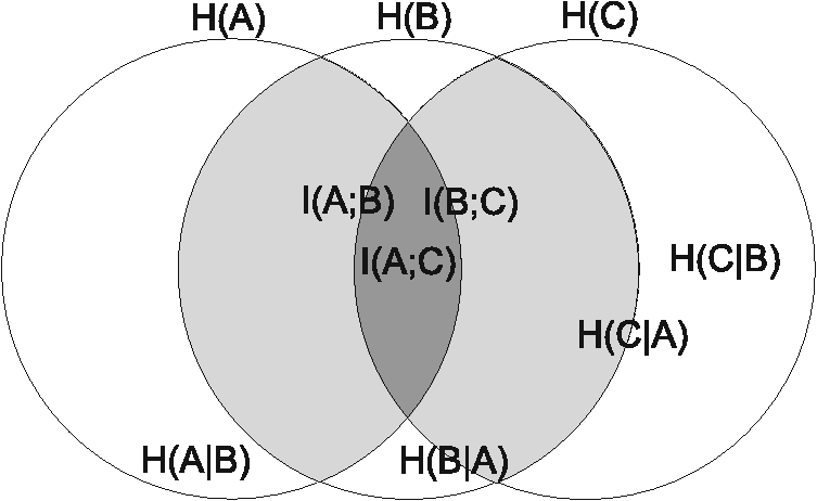

The problem can be stated in terms of rate-distortion theory³¹ and constitutes what is denoted as information-theoretic assessment.^16–18 When the source $A$ is corrupted by the instrumental noise to yield the observed source, $B$, its entropy $H(A)$ is partly lost. $H(A|B)$ is the part of $H(A)$ that gets lost after noise addition, if $A$ is no longer available and only the noisy source $B$ is known. $H(A|B)$ is usually referred to as equivocation. The mutual information between $A$ and $B$, $I(A;B)$, which is the part of the entropy of $A$ that is contained in $B$ [graphically, the intersection of the spheres $H(A)$ and $H(B)$], is calculated as

The term $H(A)$ is generally unknown, but the entropy of $B$, $H(B)$, may be estimated by compressing the available observed source (raw data) without any loss, e.g., by means of an advanced DPCM compressor. Once the noise of $B$ has been modeled and measured, the irrelevance $H(B|A)$ can be estimated as the entropy of the noise realization, which is unrelated to the spectral information, $H(A)$. $I(A;B)$ can be calculated by simply decrementing $H(B)$ by the irrelevance $H(B|A)$. Finding $I(A;B)$ is the object of the information-theoretic assessment of an acquisition system,¹⁷ because $I(A;B)$ represents the mean amount of useful “spectral” information coming from $A$ that is contained in $B$ and, if compression is strictly lossless, also in $C$, because in that case $C=B$.

Now, let us consider the lossy case, i.e., $C\ne B$. The lossy compression BR achieved by an optimized coder will approximate the mutual information between $B$ and $C$, $I(B;C)$. It is noteworthy that $I(A;B)\ge I(A;C)$, the equality holding for reversible compression only. The term $I(A;C)$ may be estimated from the noise model and measurements of $B$ and from the model of the noise introduced by the irreversible compression process, assumed to be Gaussian for lossy compression or uniformly distributed for near-lossless compression. Eventually, $H(A)$, whenever of interest, can be estimated by following the procedure described in Refs. 16 and 17.

5.

Simulation Results

5.1.

Synthetic Data

The proposed model has been first assessed on simulated noisy data. A test remote sensing image has been derived from a very high-resolution aerial photograph [pixel spacing 62.5 cm, $8192\times 8192\text{pixels}$, 8 bits per pixel (bpp)] by averaging $16\times 16$ blocks of pixels. The final pixel size is approximately 10 m. The averaging process abates the acquisition noise by over 20 dB, in such a way that the resulting image ($512\times 512$ in size, 8 bpp) may be assumed as noise-free. Additive white Gaussian noise, spatially uncorrelated having ${\sigma }_w=2$ and ${\sigma }_w=5$, has been superimposed on the test image to yield two noisy versions, having SNR [Eq. (4)] equal to 29.41 and 21.45 dB, respectively. Noisy pixel values are rounded to integers and clipped between 0 and 255. The original test image and its noisy version with ${\sigma }_w=5$ are portrayed in Fig. 4.

Fig. 4

Test images for information-theoretic assessment: (a) Noise-free original. (b) Noisy version with additive white Gaussian noise having ${\sigma }_w=5$.

The optimized two-dimensional compression method is fuzzy matching pursuits encoder (FMP),³² which employs a parametrically tunable entropy coding³³ and approaches the ultimate compression more and more closely as the computational cost increases. The BR of the noise-free image, by definition equal to the entropy of the noise-free source, is $H(A)=4.97\mathrm{bpp}$. As it appears from Fig. 4, the test image is highly textured and thus hard to compress. For each of the two noisy versions, the following amounts have been calculated varying with the allowed maximum absolute distortion (MAD), $ϵ$:

• 1. $I(B;C)$ by compressing the noisy image $B$, with $ϵ=0,1,\cdots$;

• 2. $H(C)$ by reversibly compressing the image $C$, obtained by decompressing the bit stream at point 1, for $ϵ=0,1,\cdots$;

• 3. $H(C|A)$ by taking the pixel-by-pixel difference between $B$ and $C$ (compression noise), adding it to the synthetic noise realization quantized to integer (instrument noise), and reversibly compressing the outcome, for $ϵ=0,1,\cdots$;

• 4. $I(A;C)=H(C)-H(C|A)$, for $ϵ=0,1,\cdots$.

All the information parameters defining the model are plotted in Fig. 5 for the two noisy image versions. By watching the lossless case ($ϵ=0$), we can notice that the presence of the noise makes the original information $H(A)$ (almost 5 bpp) produce a mutual information $I(A;B)$ slightly higher than 2 bpp for ${\sigma }_w=2$ and 1 bpp for ${\sigma }_w=5$. In substance, the blue plot [$I(B;C)$] represents what we pay in terms of compression BR, and the red plot [$I(A;C)$] represents what we get in terms of useful (spectral) information. It is noteworthy that $I(A;C)$ vanishes for $ϵ=6$ in the less noisy version of Fig. 5(a) and for $ϵ=4$ in the noisier version of Fig. 5(b). It seems that the compression BR is first allocated to compress the noise with MAD equal to $ϵ$. Only if such a BR is high enough is the leftover part devoted to the spectral information.

Fig. 5

Entropy and mutual information parameters estimated from compression bit rates, simulated noise realization, and true map of compression-induced errors: (a) Noisy version with ${\sigma }_w=2$. (b) Noisy version with ${\sigma }_w=5$.

5.2.

AVIRIS 2006 Data

A set of calibrated and raw images acquired in 2006 by AVIRIS has been provided by NASA/Jet Propulsion Laboratory to the Consultative Committee for Space Data Systems and is available for compression experiments. This dataset consists of five 16-bit calibrated and geometrically corrected images and the corresponding 16-bit raw images, not yet diminished by the dark signal, acquired over Yellowstone, Wyoming. Each image is composed of 224 bands and each scene (the scene numbers are 0, 3, 10, 11, 18) has 512 lines.⁷ All data have been clipped to 14 bits (a negligible percentage of outliers has been affected by clipping) and remapped to 12 bits to simulate a space-borne instrument, e.g., Hyperion. Figure 6 portrays a sample band (#20, wavelength between green and red).

Fig. 6

Sample band (#20) of AVIRIS 2006 Yellowstone scene 10.

The operational steps for implementing the proposed rate-distortion model for quality assessment of on-board near-lossless compression are the following:

• 1. Take a raw (uncalibrated) hyperspectral sequence.

• 2. Measure its noise variance (both signal-independent and signal-dependent terms) for each spectral band.

• 3. Extract the spatial noise pattern of each band, by applying a denoising filter, e.g., Ref. 34, and take the difference between original and denoised band.

• 4. Compress the sequence with the desired loss (e.g., $ϵ=0,1,\cdots$) by means of an optimized coder in order to estimate $I(B;C)$ [for $ϵ=0$, $I(B;C)=H(B)$].

• 5. Decompress the compressed sequence and compress the outcome without loss, to obtain $H(C)$, for $ϵ=1,2,\cdots$ [for $ϵ=0$, $H(C)=H(B)$].

• 6. Take the difference between original and decompressed band, i.e., the pattern of compression-induced pixel error values, for $ϵ=1,2,\cdots$.

• 7. Add the two patterns of instrumental noise and of compression errors to yield the overall error map, for $ϵ=1,2,\cdots$ [for $ϵ=0$, the map is equal to the error pattern at step 3].

• 8. Reversibly compress the overall error map to estimate $H(C|A)$, for $ϵ=1,2,\cdots$ [for $ϵ=0$, $H(C|A)=H(B|A)$].

• 9. Calculate $I(A;C)$ as $I(A;C)=H(C)-H(C|A)$, for $ϵ=0,1,\cdots$.

The noise standard deviation has been measured for Yellowstone 10 (clipped above 14 bpppb and remapped to 12 bpppb) by using the algorithm described in Ref. 35 and is reported in Fig. 7(a). Apart from marked increments at the edges of the spectral interval due to loss of sensibility of instruments, the noise standard deviation is approximately constant and always $>1.2$. The average is $\sim 1.7$. However, only the electronic, or dark, component of the noise is reliably estimated because of the presence of the dark signal, which is usually removed on ground. The photon component is undetermined because bright areas do not produce appreciable clusters in the variance-to-mean scatterplot. The photon noise variance is expected to be lower than the electronic one for whisk-broom instruments, as AVIRIS is, but not for push-broom ones, at least in visible-near infrared (V-NIR) wavelengths.^29,30

Fig. 7

AVIRIS 2006 Yellowstone scene 10: (a) Measured noise standard deviation (thermal/electronic component only). (b) Bit rate, in bits per pixel per band (bpppb), produced by the S-RLP codec.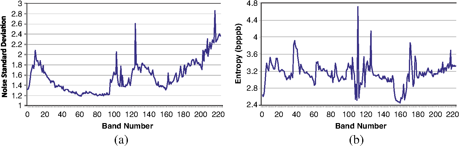

Figure 7(b) reports lossless compression BRs of AVIRIS 2006 Yellowstone raw scene 10 (clipped and remapped, as above). The compression algorithm is spectral-relaxation labeled predictor (S-RLP),⁶ which is an MAD-bounded, i.e., near-lossless algorithm, providing the ultimate compression attainable for hyperspectral data. In a possible on-board implementation, MMSE Adaptive-DPCM (MA-DPCM),³⁶ a simplified version of S-RLP, would be preferable. However, S-RLP is used only to measure the entropy of the various sources and is not required for a practical implementation.

Let $ϵ$ denote the maximum absolute reconstruction error, also known as MAD or peak error. The maximum quantization step size $\mathrm{\Delta }$ yielding MAD equal to $ϵ$ is $\mathrm{\Delta }=2ϵ+1$ and a quadratic distortion

Eq. (6)

$$D=\frac{{\mathrm{\Delta }}^2-1}{12}=\frac{{(2ϵ+1)}^2-1}{12}=\frac{4{ϵ}^2+4ϵ}{12}=\frac{ϵ(ϵ+1)}{3},$$

in which the term $({\mathrm{\Delta }}^2-1)/12$ replaces ${\mathrm{\Delta }}^2/12$ whenever real values that have been previously quantized to integers are requantized with an integer step size $\mathrm{\Delta }>1$.

Figure 8 reports information parameters for the whole sequence of Yellowstone 10. Absorption bands, in which the model of noisy information source does not hold because the spectral signal is practically zero and only noise and dark signals are present, are removed before averaging the information measures over the spectral bands (all bands are compressed).

Fig. 8

Estimated entropy and mutual information parameters for AVIRIS 2006 Yellowstone 10, whole sequence.

When $ϵ=0$, $C=B$, hence $I(B;C)=I(B;B)=H(B)$. $I(B;C)$ is monotonically decreasing with the mean quadratic distortion, or better with the quantization step size $\mathrm{\Delta }=(2ϵ+1)$, approximately as $I(B;C)=H(B)-{\log }_2(\mathrm{\Delta })$. $H(C)$ depends on how much $C$ has been smoothed by the lossy compression of $B$, or in other words on how the compression algorithm works. The term $H(C|A)$ represents the entropy of the sum of the two events, both independent of $A$, that are acquisition noise and compression errors, which have been verified to be independent of one another for DPCM compression in the tests on simulated data. Given the BRs produced by the optimized encoder S-RLP, CRs can be calculated relative to the uncompressed wordlength of 12 bits. The CR versus MAD characteristic of the actual on-board DPCM coder will be likely to yield a slightly lower CR.

The analysis reported suffers from a main shortcoming. Photon noise has been disregarded since its estimation is difficult, also because of the presence of the dark signal, which is not to be considered in the model [Eq. (2)]. Actually the SNR of AVIRIS 2006 data is extremely high (over 50 dB, in average), which means that the noise is so weak that it can be reliably estimated only on the lake. Since the average level of the lake is significantly lower than the average level of the whole band, a non-negligible fraction of the photon noise term is neglected. However, the error on the overall noise variance estimation is expected to be $<10\%$ by defect. In this case, the mutual information $I(A;C)$ would be overestimated by $<0.05\mathrm{bpppb}$.

In a practical application scenario, suppose you cannot afford onboard lossless compression and you have to use lossy compression. For a sample hyperspectral raw image, the method provides the amount of useful spectral information $I(A;B)$, that is, information pertaining to the noise-free source and not the acquired noisy source, varying with the amount of distortion introduced by compression on the acquired noisy source. On the other side, distortion can be related to CR or coding BR, through the rate distortion (RD) characteristic of the coder used in the actual implementation, i.e., on-board. So, the coder can be designed to preserve a specified amount of information and not to yield a specified amount of distortion, as happens most usually. The proposed method can be applied to existing systems, provided that they use DPCM with quantization step sizes that can be uploaded from ground and allow lossless compression to be performed as a limit case. The procedure is summarized by the following steps:

• 1. Download a sample lossless scene.

• 2. Measure its noise, or use laboratory noise measurements of the instrument.

• 3. Run the model on the lossless scene.

• 4. Find the maximum absolute error, and hence the quantization step size, that yields the desired amount of $I(A;C)$.

• 5. Upload the step size to the satellite system.

• 6. Use such step size to produce compressed data having the desired amount of spectral information.

6.

Concluding Remarks

This study has proposed a rate-distortion model to quantify the loss of useful spectral information that gets lost after near-lossless compression, and its experimental setup, such that the information-theoretical model may become a computational model. The key ingredient of this recipe is an advanced hyperspectral image coder providing the ultimate compression regardless of time and computation constraints (such a coder is not necessary to perform on-board compression, but only for simulations). Noise estimation is crucial because of the extremely low noisiness of hyperspectral data that are also richly textured. Noise filtering is also required to extract noise patterns. The drawback is that denoising filters generally work properly if they know reasonably exact values of the parameters of the noise model they have been designed for. Preliminary results on AVIRIS 2006 Yellowstone 10 sequence are encouraging, although absorption/anomalous bands are likely to contradict the main assumptions underlying the proposed model and should not be considered. The main conclusion that can be drawn is that the noisier the data, the lower the CR that can be achieved in order to retain a prefixed amount of spectral information. This happens because the noise-free data can tolerate up to a certain amount of cumulative noise, i.e., instrument noise plus compression-induced noise. Thus, if instrument noise is higher, compression noise shall be lower, and vice versa.