|
|
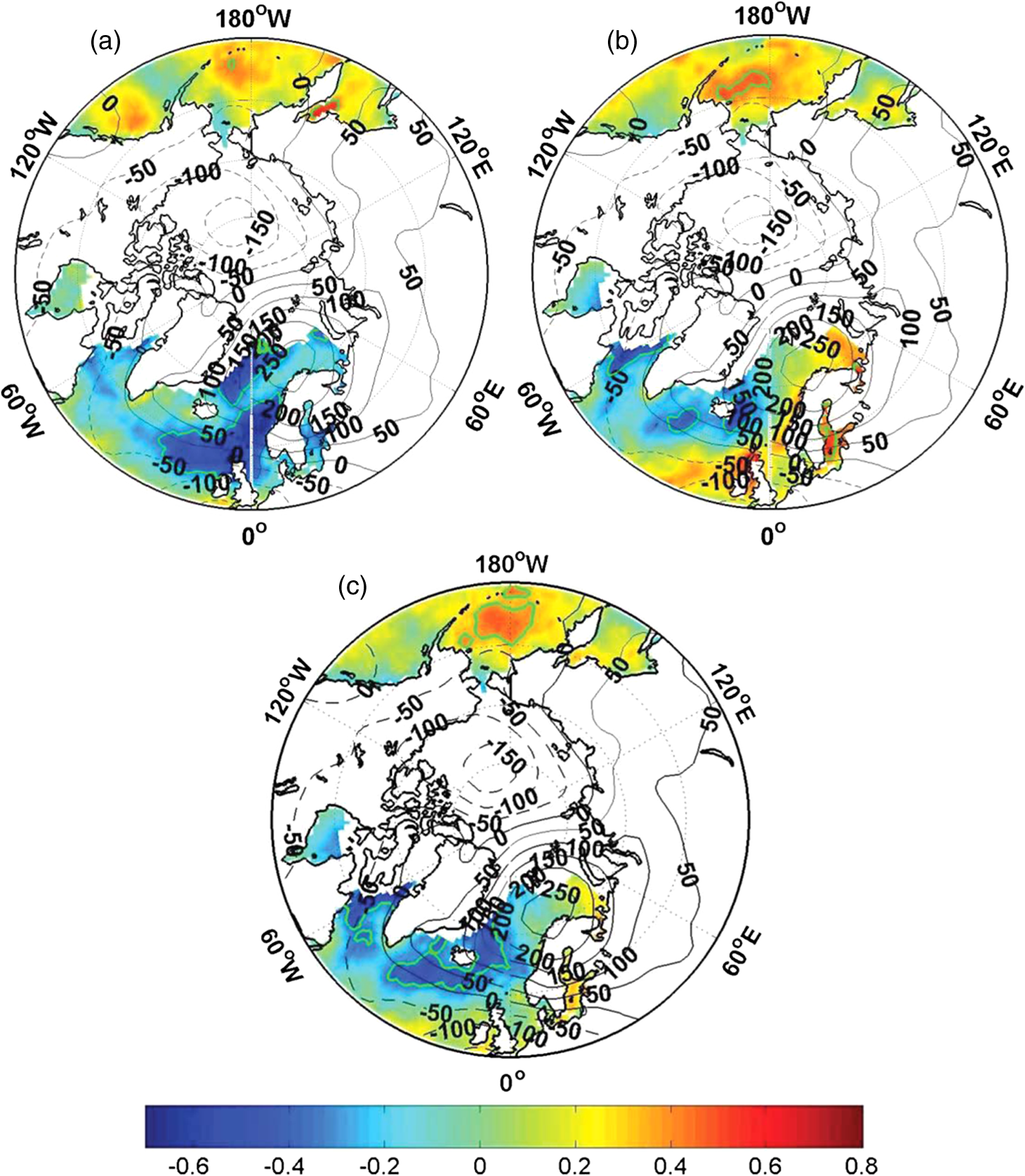
1.IntroductionLatent and sensible heat fluxes (LHF and SHF) at the ocean surface are the dominant mechanism for transferring heat from ocean to atmosphere, and their importance to the general circulation of the atmosphere has long been recognized. The amount of LHF and SHF and their distribution over the global oceans are required for climate research. In recent decades, the Arctic sea ice and sea surface temperature (SST) have apparently changed.1,2 Gill and Niiler3 revealed that over large scales, surface temperature changes are dominated by changes in surface heat fluxes including LHF and SHF, in comparison with advective influences. The roles of both LHF and SHF in the changes of the Arctic sea ice and SST need to be investigated. Hence, it is necessary to obtain trends in LHF and SHF in the Arctic regions and their relationships with surface atmospheric variables. Several large-scale circulation indices impact the atmospheric and oceanic environment over the Arctic regions. The Arctic Oscillation (AO) is the leading empirical orthogonal function (EOF) of monthly and seasonal extratropical sea level pressure (SLP) anomalies in the Northern Hemisphere characterized by deep, zonally symmetric structures.4 The North Atlantic Oscillation (NAO), which is the Atlantic section of the AO,5 influences greatly the LHF and SHF over the northern Atlantic Ocean. Cayan6 found that when the NAO is in its strong Icelandic low phase, positive anomalous LHF and SHF occur east of Labrador, south of Greenland, and off the coast of Africa; negative anomalous LHF and SHF occur offshore of the United States just north of Bermuda. Cayan6 also found that the Pacific-North American (PNA) pattern has a positive correlation with LHF and SHF over a broad region southwest of the Aleutian low and a negative correlation over the region east of the Aleutian low along the west coast of the United States. The second EOF of the SLP north of 70°N is denoted as the Arctic dipole anomaly (DA), which is an important driver of the Arctic sea ice transport from the western Pacific Arctic to the northern Atlantic Arctic based on data analysis for the period 1962 to 2002.7 The third mode (PC3) refers to a seesaw structure in SLP anomalies between the Barents Sea and the Beaufort Sea, which influences Fram Strait sea ice flux.8 The second mode EOF of monthly winter SLP anomalies poleward of 30°N, called the Barents Oscillation (BO), has a high temporal correlation with the sensible heat loss from the Nordic Seas.9 Cayan6 reported that the two leading EOFs of SLP are the NAO and the Eastern Atlantic (EA) pattern in the North Atlantic,10 and PNA and the Bering Sea (BER) pattern11 in the North Pacific, respectively. Among the four indices, the EA and BER indices are correlated with the PC3 index with above 95% confidence. In addition, a significant correlation also occurs between the DA and BO indices. Hence, this article investigates the extent to which the AO, DA, PC3, and PNA can account for the recent trends in LHF and SHF over the oceans surrounding the Arctic Ocean, together with the contribution of surface meteorological variables. The article is arranged as follows: Sec. 2 describes the data sources and analytical methods. Section 3 discusses the results, and the conclusions are given in Sec. 4. 2.Data and MethodsThe monthly LHF and SHF are derived from the Objectively Analyzed air-sea Fluxes (OAFlux) dataset with a spatial resolution of from January 1979 to December 2008.12 The positive fluxes are defined upward. To obtain the best possible global daily estimates for wind speed at 10 m, SST, and air temperature and humidity at 2 m, the OAFlux synthesis uses surface meteorological fields derived from satellite remote sensing and reanalysis outputs produced from the National Centers for Environmental Prediction (NCEP) and the European Centre for Medium-Range Weather Forecasts (ECMWF) models.13 Satellite products in the OAFlux synthesis include wind speed retrievals from both active (scatterometer) and passive (radiometer) microwave remote sensing, and SST daily high-resolution blended analysis by Reynolds et al.14 The synthesis includes also the near-surface humidity product derived by Chou et al.15 from the Special Sensor Microwave Imager column water vapor retrievals. The OAFlux project uses the state-of-the-art Coupled Ocean Atmosphere Response Experiment (COARE) bulk flux algorithm version 3.016 to compute the fluxes. Yu et al.13 indicated that the OAFlux estimates are unbiased and have a smaller mean error than NCEP1, NCEP2, and ECMWF. In addition, OAFlux data for wind speed at 10 m, humidity at 2 m, and SST are also used. The AO, DA, and PC3 indices are defined as the standardized leading three modes of EOF analysis of monthly SLP poleward of 70°N. The PNA index is obtained from the website http://jisao.washington.edu/data/pna/. The total linear trends are obtained from a least square linear fit at each grid point at specific periods. The trends that are linearly congruent with the monthly AO, DA, PC3, and PNA indices can be obtained in the following manner:4
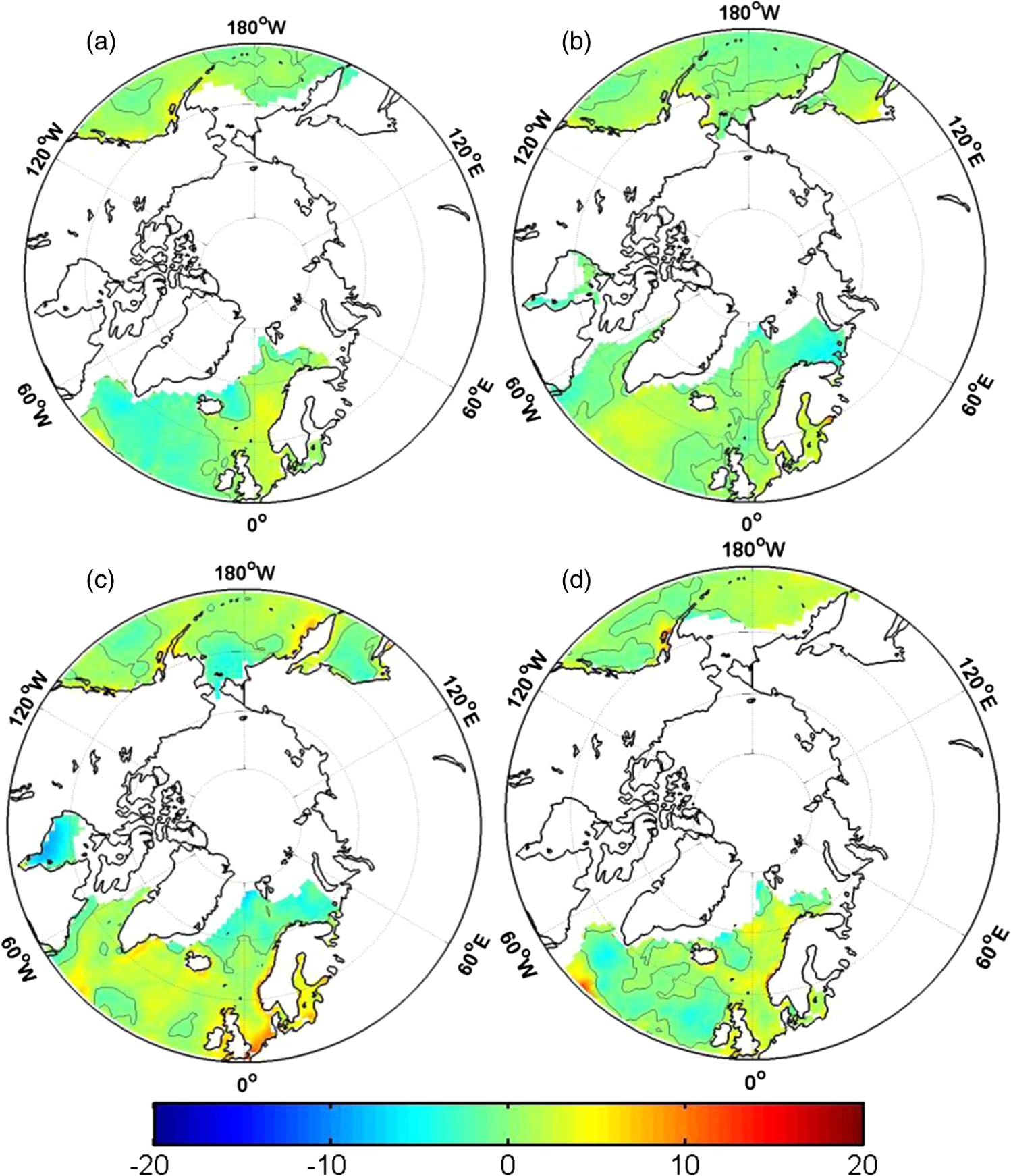
Residual trend is defined as the trend obtained by subtracting the trends in the AO, DA, PC3, and PNA indices from the total trend. 3.Results3.1.Trends of LHF and SHFThe trends of LHF over the oceans surrounding the Arctic Ocean for the four seasons are shown in Fig. 1. In spring [Fig. 1(a)], LHF over the northern Pacific regions has a positive trend over the coast of the Gulf of Alaska and a negative trend offshore of the Kamchatka Peninsula; over the northern Atlantic regions, we see a positive trend over the Norwegian Sea and the North Sea, and a negative trend over the regions south of Greenland and northeast of Iceland. Elsewhere a positive trend occurs offshore of Canada at 70°N. The LHF trend in spring is the smallest among the seasons, from to . Fig. 1Trends of LHF over the oceans surrounding the Arctic Ocean. (a) spring; (b) summer; (c) autumn; (d) winter. Units are . The thin lines indicate the regions of confidence level.  In summer [Fig. 1(b)] over the northern Pacific regions, a significant positive trend occurs over the Sea of Okhotsk, but the area of positive trend over the Gulf of Alaska decreases. A small patch of negative trend appears over the Bering Sea, the Gulf of Alaska, and the region southwest of the Aleutian Islands. Most of the North Atlantic region shows a positive trend in LHF and a negative trend over the Barents Sea, the coast of northeast Canada, and Hudson Bay. The trend in LHF from to in summer is larger than that in spring as a result of increasing sea temperature. In autumn [Fig. 1(c)], the main negative trend occurs over the Bering Sea, the Sea of Okhotsk and Hudson Bay, where the largest negative trend is . A positive trend occurs over the coast of the Kamchatka Peninsula, the Aleutian Islands, and northern and western Europe. The largest positive trend of appears on the Netherlands coast, possibly because the cold land and warm sea lead to a larger sea–air humidity difference near the coast. In winter [Fig. 1(d)], no significant negative trend occurs over the northern Pacific and Atlantic regions. A positive trend is situated over the eastern part of the northern Pacific Ocean and the coast of Norway. Elsewhere the largest positive trend of occurs offshore of Canada at 70°N influenced mainly by the North Atlantic Current. The trend in SHF over the northern Pacific and Atlantic regions is shown in Fig. 2. In spring, the trend pattern is similar to LHF, but the negative trend in LHF south of Greenland is less significant than in SHF with a maximum value of [Fig. 2(a)]. In summer over the northern Atlantic regions and the Sea of Okhotsk, the trend pattern in SHF is similar to that in LHF, but the remarkable positive trend over the Gulf of Alaska seen in LHF is not seen in Fig. 2(b). In addition, the magnitude of the trend in SHF is less than that in LHF. The autumn trend in SHF has a pattern similar to that in LHF with the exception of a slight difference in magnitude [Fig. 2(c)]. The largest change of SHF occurs in winter, ranging from to , but the area is confined to the oceans northwest of Ireland and northeast of Iceland, Fram Strait, the Barents Sea, and the northern Bering Sea [Fig. 2(d)]. 3.2.Relationships Between LHF and SHF and the IndicesTo explore the relationships between LHF and the four indices, correlations between the four indices and the grid point fields of wind speed, sea–air-specific humidity difference and LHF in autumn are superimposed on the patterns of the four indices in Figs. 3Fig. 4Fig. 5–6, respectively. In Fig. 3(a), when the SLP anomaly at high latitudes is positive, less frequent storms lead to lower wind speed in the northeast Atlantic Ocean.6 Similarly, the pattern in the northern Pacific region is a zonal dipole structure, that is, the wind speed increases over the Sea of Okhotsk and decreases over the Gulf of Alaska and the Bering Sea. Fig. 3Correlation coefficients, spatial patterns of the AO index versus all grid point time series of wind speed (a), sea–air-specific humidity difference (b), and LHF (c) in autumn from 1979 to 2008. Thin contours show the patterns of the AO index. The thick solid green lines indicate the regions of confidence level. 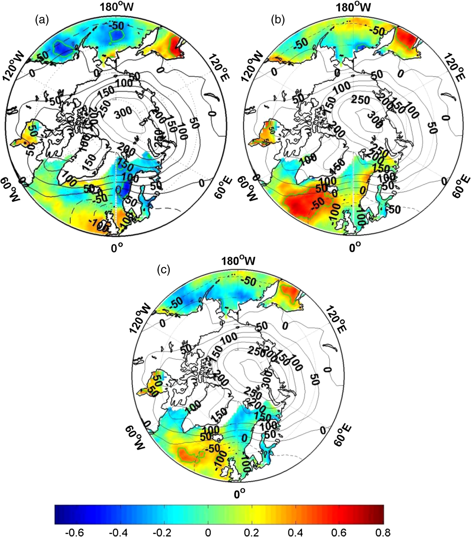 The relationship between the SLP and air–sea-specific humidity difference is similar to that of the SLP and wind speed only in the Sea of Okhotsk [Fig. 3(b)]. The other positively correlated region lies south of Greenland and Iceland. A small patch of negative correlation lies northwest of the Bering Sea. The pattern of air–sea-specific humidity difference is associated with wind advection. The cold dry air from northern Europe and the Kamchatka Peninsula moves toward the Sea of Okhotsk and the region south of Greenland and Iceland, whereas warm moist air moves northwest toward the Bering Sea. The cold (warm) dry (moist) air induces a greater (smaller) air–sea-specific humidity difference. The correlation pattern between AO and LHF [Fig. 3(c)] resembles more than that of the correlation of air–sea-specific humidity difference, with significant positive centers in the Sea of Okhotsk and south of Greenland at 30°W. But the regions with negative correlation of wind speed in Fig. 3(a) do not result in negative correlations of LHF in Fig. 3(c). A small negative correlation is situated on the east coast of the Bering Sea. The spatial pattern of correlation between LHF and AO is consistent with that between LHF and NAO at high latitudes.5 The correlations of the DA index with wind speed, air–sea-specific humidity difference, and LHF are quite large and very different from those with the AO index [Figs. 4(a)–4(c)]. When the pressure anomaly of the center in the Kara Sea is negative, negative correlations are scattered over the northern Pacific west of 170°W, and positive correlations occur over the Gulf of Alaska; for the northern Atlantic region, positive correlations occur over the oceans north of 60°N, and negative correlations occur between 57°N and 50°N. In Fig. 4(b), in contrast with the correlation of wind speed, the center of negative correlations between DA and air–sea-specific humidity difference in the northern Atlantic region moves eastwards near the coast of Ireland and that of positive correlation shrinks northwards. In the northern Pacific region, the negative correlations are confined to the western Sea of Okhotsk. The pattern of the correlation of LHF with DA partially resembles both of the above but is more similar to that of air–sea-specific humidity difference in the northern Atlantic regions. But the region with negative correlation of LHF in the northern Pacific is larger than that of air–sea-specific humidity difference and wind speed. The two variables also influence the relationships between LHF, and PC3, and PNA (Figs. 5 and 6) When the Barents Sea is in the positive phase, a significantly positive correlation occurs over the Bering Sea, and a negative correlation occurs over the Davis Strait and the seas surrounding Iceland. When the circulation is in its strong Aleutian low phase, the cold and dry air from land and the warm and moist air from sea bring about a positive correlation in the region southwest of the Aleutian Islands and a negative correlation over the Gulf of Alaska, which agrees with the result of Cayan.6 A positive correlation also exists over Hudson Bay and the northern Atlantic Ocean south of 70°N. The relationships between the four indices and SHF in autumn are similar to those between the four indices and LHF, and the pattern of SHF caused by the four indices is associated with that of wind speed and air–sea temperature difference. In other seasons, the relationships between the four indices and both LHF and SHF are similar to those in autumn with the exception of the difference in correlation coefficients. Similar explanations of these relationships in autumn also apply to those in other seasons. 3.3.Contributions of the IndicesThe different seasonal trends in the AO, DA, PC3 and PNA indices can produce different impacts on the trends in LHF and SHF among seasons. In this subsection, we investigate the contributions of the four indices to the seasonal trends in LHF and SHF over the northern Pacific and Atlantic regions. Due to the more remarkable change of LHF and the extensive open water in autumn, only the patterns of autumn LHF caused by the four indices are shown in Fig. 7. When the AO index shows a decreasing trend of 0.77 SD per 30 years, the positive trends occur mainly over the Gulf of Alaska, the Bering Sea, the Davis Strait, the Norwegian Sea, the Greenland Sea, and the Baltic Sea; the negative trends are over the Sea of Okhotsk, the southern Hudson Bay, and the southern part of the northern Atlantic Ocean. The maximum value of is over the Gulf of Alaska, and the minimum value of is over southern Hudson Bay. The structure of the pattern has been explained in the previous subsection. In the same 30 year period, the positive trend of DA with the value of 0.76 SD per 30 years leads to the change in LHF from to . The maximum value occurs in the Greenland Sea, the minimum value offshore of Ireland. The impact of PC3 on the trend in LHF is the least among the four indices with less than half of that caused by DA. The negative change in LHF caused by PNA appears mainly in the Gulf of Alaska with the minimum value of . Most of the northern Atlantic Ocean, the Sea of Okhotsk, and the sea surrounding the Aleutian Islands display increasing trends of LHF with a maximum value of . Fig. 7Trends of autumn LHF associated with (a) AO; (b) DA; (c) PC3; (d) PNA. Units are . The solid thin lines indicate the value of 0.  The pattern of the trends in LHF caused by the four indices among other seasons is similar to that in autumn, with some differences in sign and magnitude. Among the four indices, the impact of DA on the trend in LHF is the largest among seasons. In spring and summer, the contribution of AO to the trend in LHF is smallest, but in autumn and winter, the least effect comes from PC3. For the four indices, their contributions to the trend in LHF show some seasonality, especially for AO and PC3, whose contributions in autumn and winter are more significant than that in spring and summer. The spatial structure of the trend in SHF related to the four indices is nearly the same as that of LHF, but the magnitude of the trend is different (not shown). Like LHF, DA exerts the strongest effect on the long-term change of SHF, and in spring and summer, the smallest contributor is AO; in other seasons, it is PC3. Compared to LHF, the range of the trend in SHF related to the indices is larger in spring, autumn, and winter but smaller in summer. 3.4.Residual TrendsResidual trends, which reflect the trends that cannot be explained by the four indices, are shown in Fig. 8. The spatial patterns of residual trends are similar to those of total trends in Fig. 1. The largest residual trend in LHF occurs over the ocean south of Greenland and the Norwegian Sea in spring, over the Barents Sea and southern Hudson Bay in summer, over Hudson Bay and the coast of West Europe in autumn; and it is scattered in the northern Atlantic Ocean in winter. The residual trend in SHF has the same characteristics as LHF (Fig. 8). Hence, the similarity between the residual and total trends in LHF and SHF indicates that other factors may contribute mainly to the trends in LHF and SHF. 3.5.Trends of Other Meteorological VariablesBecause the trends in LHF and SHF are less affected by the main large-scale circulation indices, we seek the explanation in meteorological variables. The trends in air–sea-specific humidity difference, 10-m wind speed, and air–sea temperature difference are shown in Figs. 9Fig. 10–11. The spatial patterns of the trends in air–sea-specific humidity difference are similar to those of LHF among seasons (Fig. 9) but with some small differences. In summer, the significant increasing trend in LHF in the region south of Greenland does not correspond to the remarkable increasing trend in air–sea-specific humidity difference in the same region. In autumn, the extent of the significantly negative trends of air–sea-specific humidity difference exceeds that of LHF in the Okhotsk Sea. The spatial patterns of the trends in wind speed among seasons are not consistent with those of LHF, especially over the central North Atlantic Ocean in summer. But along some coasts, for example, the coasts of the Gulf of Alaska and North Europe, and the southern Hudson Bay, they show a certain consistency. According to the bulk parameterization of LHF, apart from wind speed and air–sea-specific humidity difference, aerodynamic transfer coefficient can also influence LHF. Moreover, the aerodynamic transfer coefficient is related to wind speed, and their relationship is nonlinear and complicated.16 Hence, the consistency of wind speed and LHF is various depending on the time and circumstances. The 30-year trends in air–sea temperature difference are shown in Fig. 11. The similarity of the spatial patterns of the trends between air–sea temperature difference and SHF is more remarkable than that between air–sea-specific humidity difference and LHF. The air–sea temperature difference is larger for larger SHF. But compared to the trend in air–sea temperature difference, wind speed cannot show a consistent trend with SHF, especially in the summertime North Pacific and Atlantic. Like LHF, decreasing trends in wind speed and SHF occurs over the southern Hudson Bay. According to previous research,17,18 not only wind speed but also the atmospheric stable condition measured by the Richardson number can influence the aerodynamic transfer coefficient for heat. Hence, the trends in aerodynamic transfer coefficient need to be explored further. 4.ConclusionsIn this study, the trends in LHF and SHF over the oceans surrounding the Arctic Ocean were investigated using the OAFlux dataset from 1979 to 2008. Additionally, the contributions of the AO, DA, PC3, and PNA indices to the trends in SHF and LHF, and the impacts of air–sea-specific humidity difference, wind speed, and air–sea temperature difference were also considered. Among the seasons, the mainly positive trends in LHF occur over the coast and the ocean south of Greenland, and the mainly negative trends occur over Hudson Bay, the Barents and Bering Seas, and the coast of Canada. The ranges of the trends in LHF in autumn and winter exceed those in spring and summer. Among seasons, the spatial patterns of the trends in SHF are not in agreement with those of LHF, especially over the summertime northern Pacific region. The range of the trends in SHF in winter, which is the largest among the seasons, is from to . Through correlation analysis, we find strong relationships between the four indices and both LHF and SHF in the northern Pacific and Atlantic regions. The relationships can be explained by the wind speed and air–sea-specific humidity and temperature differences. Among these variables, air–sea-specific humidity and air–sea temperature differences are more important than wind speed. The four indices make a smaller contribution to the trends in LHF and SHF although the wintertime DA leads to a change of SHF from to . Spatial patterns of the residual trends in LHF and SHF are similar to total trends of LHF and SHF. However, other explanations for the residual trends should be investigated, e.g., local factors. The trends in air–sea-specific humidity difference and temperature difference can account for those in LHF and SHF over the 30 years although in some regions, the trend in wind speed also influences LHF and SHF. Due to the uncertainty of the effect of wind speed on aerodynamic transfer coefficient, the consistency between wind speed and heat fluxes is broken. The trends in aerodynamic transfer coefficient for heat need to be investigated in the future. AcknowledgmentsThis study was supported by the National Natural Science Foundation of China 41175010, 41106164 and 40930848 and Marine Public Welfare Project (201205007). The National Center for Atmospheric Research is sponsored by the National Science Foundation. ReferencesM. M. HollandC. M. Bitz,
“Polar amplification of climate change in coupled models,”
Clim. Dyn., 21
(3–4), 221
–232
(2003). http://dx.doi.org/10.1007/s00382-003-0332-6 CLDYEM 0930-7575 Google Scholar
O. M. Johannessenet al.,
“Arctic climate change: observed and modeled temperature and sea-ice variability,”
Tellus, 56A
(4), 328
–341
(2004). TELLAL 0040-2826 Google Scholar
A. E. GillP. P. Niiler,
“The theory of the seasonal variability in the ocean,”
Deep Sea Res., 20
(2), 141
–177
(1973). http://dx.doi.org/10.1016/0011-7471(73)90049-1 Google Scholar
D. W. J. ThompsonJ. M. Wallace,
“Annular modes in the extratropical circulation. Part I: month-to-month variability,”
J. Clim., 13
(3), 1000
–1016
(2000). http://dx.doi.org/10.1175/1520-0442(2000)013<1000:AMITEC>2.0.CO;2 JLCLEL 0894-8755 Google Scholar
M. H. P. AmbaumB. J. HoskinsD. B. Stephenson,
“Arctic oscillation or North Atlantic oscillation?,”
J. Clim., 14
(16), 3495
–3507
(2001). http://dx.doi.org/10.1175/1520-0442(2001)014<3495:AOONAO>2.0.CO;2 JLCLEL 0894-8755 Google Scholar
D. R. Cayan,
“Latent and sensible heat flux anomalies over the northern oceans: the connection to monthly atmospheric circulation,”
J. Clim., 5
(4), 354
–369
(1992). http://dx.doi.org/10.1175/1520-0442(1992)005<0354:LASHFA>2.0.CO;2 JLCLEL 0894-8755 Google Scholar
B. WuJ. WangJ. E. Walsh,
“Dipole anomaly in the winter Arctic atmosphere and its association with Arctic sea ice motion,”
J. Clim., 19
(2), 210
–225
(2006). http://dx.doi.org/10.1175/JCLI3619.1 JLCLEL 0894-8755 Google Scholar
B. WuM. A. Johnson,
“A seesaw structure anomalies between the Beaufort Sea and the Barents Sea,”
Geophys. Res. Lett., 34
(5), L05811
(2007). http://dx.doi.org/10.1029/2006GL028333 GPRLAJ 0094-8276 Google Scholar
P. Skeie,
“Meridional flow variability over the Nordic seas in the Arctic Oscillation framework,”
Geophys. Res. Lett., 27
(16), 2569
–2572
(2000). http://dx.doi.org/10.1029/2000GL011529 GPRLAJ 0094-8276 Google Scholar
A. G. BarnstonR. E. Livezey,
“Classification, seasonality, and persistence of low-frequency atmospheric circulation patterns,”
Mon. Weather Rev., 115
(6), 1083
–1126
(1987). http://dx.doi.org/10.1175/1520-0493(1987)115<1083:CSAPOL>2.0.CO;2 MWREAB 0027-0644 Google Scholar
J. C. Rogers,
“Patterns of low-frequency sea level pressure variability (1899–1986) and associated wave cyclone frequencies,”
J. Clim., 3
(12), 1364
–1379
(1990). http://dx.doi.org/10.1175/1520-0442(1990)003<1364:POLFMS>2.0.CO;2 JLCLEL 0894-8755 Google Scholar
L. YuR. A. Weller,
“Objectively analyzed air-sea heat fluxes for the global ice-free oceans (1981–2005),”
Bull. Am. Meteor. Soc., 88
(4), 527
–539
(2007). http://dx.doi.org/10.1175/BAMS-88-4-527 BAMIAT 0003-0007 Google Scholar
L. YuX. JinR. A. Weller,
“Multidecade global flux datasets from the Objectively Analyzed air-sea Fluxes (OAFlux) Project: latent and sensible heat fluxes, ocean evaporation, and related surface meteorological variables,”
8
–14
(2008). Google Scholar
R. W. Reynoldset al.,
“Daily high-resolution-blended analyses for sea surface temperature,”
J. Clim., 20
(22), 5473
–5496
(2007). http://dx.doi.org/10.1175/2007JCLI1824.1 JLCLEL 0894-8755 Google Scholar
S.-H. Chouet al., Goddard Satellite-based Surface Turbulent Fluxes (GSSTF)—Version 2 Documentation, 11
–14 Distributed Active Archive Center (DAAC), NASA Goddard Space Flight Center, Greenbelt, Maryland
(2001). Google Scholar
C. W. Fairallet al.,
“Bulk parameterization of air-sea fluxes: updates and verification for the COARE algorithm,”
J. Clim., 16
(4), 571
–591 2003). Google Scholar
S. K. EsbensenR. W. Reynolds,
“Estimating monthly averaged air-sea transfers of heat and momentum using the bulk aerodynamic method,”
J. Phys. Oceanogr., 11
(4), 457
–465
(1981). http://dx.doi.org/10.1175/1520-0485(1981)011<0457:EMAAST>2.0.CO;2 JPYOBT 0022-3670 Google Scholar
J. A. CurryP. J. Webster,
“Ocean surface exchanges of heat and fresh water,”
Thermodynamics of Atmospheres and Oceans, 252
–253 Academic Press, San Diego, CA
(1999). Google Scholar
Biography Lejiang Yu is a lecturer at Nanjing University of information Science & Technology. He received his PhD degree in physical oceanography from the Institute of Oceanology, Chinese Academy of Sciences, in 2008. His current research interests include large-scale sea–air–ice interaction and monsoon dynamics. |