
|
|
1.IntroductionAerosol optical thickness (AOT) or aerosol optical depth (AOD) is a standard measure for atmospheric aerosol loading from optical remote sensing measurements and as a result, AOD has become a major atmospheric data product derived from various earth observation satellites, such as the Moderate Resolution Imaging Spectroradiometer (MODIS), the Multiangle Imaging Spectro-Radiometer (MISR), the Sea-viewing Wide Field-of-view Sensor (SeaWiFS), the Ozone Monitoring Instrument (OMI), and many others.1 These remote-sensing satellites obtain geolocated and calibrated radiances as Level 1B data, which are then input into complex retrieval algorithms to derive the corresponding AOD (Level 2) data products. Unfortunately, differences in the retrieval algorithms and/or in the instrument capabilities can introduce biases leading to different AOD values. For instance, the MODIS Dark Target Algorithm has some difficulties computing AOD in parts of its swath over dark water due to sun glint,2 whereas MISR is able to retrieve AOD under these conditions because of its off-nadir cameras.3 Even in regions where different algorithms are valid, different AOD values over the same region can occur through different algorithms (e.g., MODIS Dark Target Algorithm versus MODIS Deep Blue Algorithm) from the same satellite observational scene. Other factors which can cause inconsistencies among various AOD data sets may be due to: (a) differences in cloud masking; (b) treatment of surface boundary conditions (such as wind velocities, temperature, specific humidity, etc.) at the surface of the ocean or land; and (c) assumptions about component aerosol microphysical properties, as explained in Refs. 12.3.–4. Additional factors include instrument calibration,1,5 improper assumptions for the key elements used in the algorithms, such as aerosol type and size distribution, and sampling differences among the instruments.1,3,6 The need to treat aerosol variability in a consistent and realistic way is addressed in many studies. For example, there have been several attempts to cross-calibrate radiances and then apply the same aerosol retrieval algorithm to multisensor data, but these mostly concentrated on selected regions7,8 or on a single scene.9 Zhang and Reid10 analyzed AOD biases over oceans using Aerosol Robotic Network (AERONET) to develop specific empirical corrections and quality assurance procedures and integrate them into the operational data assimilation system. Kinne et al.11 proposed to rank aerosol measurements by different sensors and AERONET, but they compared only mean AOD values for different regions and seasons without using other statistical methods. Determination of bias in AOD is rather problematic, due to its unknown sources of errors, nonlinearity in the dataset itself, and the presence of non-normal distributions. Therefore, commonly used linear methods may not be suitable to represent the aerosol characteristics. A powerful approach to deal with these nonideal cases is to utilize a nonparametric approach where all the statistical properties of the retrieved aerosol quantity can be taken into consideration. In this study, we used a neural network (NN) as the mathematical estimator. This approach allows us to reduce (i.e., compensate for) different types of sensor and algorithm retrieval biases without the requirement of knowing the source of the systematic error in advance.12,13 The NN used for our purpose is a supervised learning algorithm defined as an application in which training data comprises examples of the input vectors along with their corresponding target vectors. If the desired output consists of one or more continuous variables, then the task is called NN regression.12 This is the meaning for the term NN used in the remainder of this article. Neural networks have been used for many different earth science applications. Examples include retrieval of land surface reflectance14 and retrieval of precipitation from microwave observations.15 In addition, direct calculation of AOD values and properties using radiance data from MODIS is described in Refs. 16 and 17. Das et al.17 applied the AOD prediction model by considering an active learning–based data collection method, which facilitated the learning of a sufficiently accurate AOD prediction model using a minimal set of labeled training data by querying the labels of only the most informative data points. Improvement in the accuracy of AOD values using data mining techniques was also studied by Han et al.18 Cazorla et al.19 applied three NN-based models using radial bases function networks to estimate the value of AOD at three different wavelengths using the radiance over the principal plane of the sky images from a calibrated sky imager. Although these studies concentrated on inputting radiance (Level 1B), Lary et al.20 applied NN directly to retrieved AOD on the basis of AERONET data. Note that NN was used in Lary et al. to adjust and/or validate the biases for MODIS AOD that were already calculated using the physical model algorithm. Although Ref. 20 introduces valuable insight to the bias adjustment problem, it uses a small number of data points during the NN training process (7543 for MODIS-Aqua and 13,034 for MODIS-Terra) which affects the assessment of the performance results. In our study, we improve both quality and volume of the training data set by using data points while also considering land and ocean bias adjustments separately. In order to use the NN method, the first step is to organize the data set into a usable form and to select the correct variables that contribute the most relevant information for the estimation process. In this work, we use highly accurate and quality-assured AERONET measurements as the ground truth (GT).21 AERONET measurements provide for one of the most precise and accurate aerosol datasets available.22 As a result, AERONET data are especially suitable for validation purposes and have been used to evaluate MODIS,2,4,23 MISR,3 and other aerosol data sets from space-based remote sensing. In applying the NN method, it is crucial to have proper training data that well represent past experiences. In this study, the training data are composed only of data possessing collocation between ground stations and satellites. For this purpose, the Multisensor Aerosol Products Sampling System (MAPSS) is used.24 This system consistently samples aerosol products from multiple space-borne sensors such as MODIS-Terra, MODIS-Aqua, MISR, Polarization and Directionality of the Earth’s Reflectances (POLDER), OMI, Cloud-Aerosol Lidar with Orthogonal Polarization (CALIOP), and SeaWiFS and collocates them with ground AERONET stations over uniform 55-km diameter ground areas that are centered on AERONET stations. For each extracted sample, MAPSS calculates a set of spatial statistics including mean, median, standard deviation, direction and rate of spatial variation, and spatial correlation coefficient. In the MAPPS database, MODIS products come with a QA flag (with discrete values of 0, 1, 2, or 3) over land and over ocean. This flag is a byproduct of the MODIS retrieval algorithm and it indicates how confident the algorithm is in a particular retrieved result. In MAPSS, mode of this flag over the sampled area is calculated.23 Furthermore, MAPSS identifies AERONET data measured within 30 min of the overpass time of each space-borne data sample and calculates a corresponding set of temporal statistics. The assumption here is that since air masses are in constant movement, an aerosol plume observed by MODIS over the 55-km sampling circle will also be observed by AERONET during the 1-h sampling period.23 In this way, MAPSS enables direct cross characterization and comparative analysis between space-borne and ground-based aerosol observations.23 Implementation of the bias adjustment algorithm based on the NN approach results in the removal of mean bias, reduction in variance in the satellite retrieved AOD data, and a better handling of the non-Gaussian distributions. The protocol adopted for our NN estimator includes (1) only the MAPSS database is used for the preparation of the training data set; (2) separate training for each satellite and product—for example, the inclusion of MISR data as regressors for MODIS training data is not allowed and ocean and land products are treated separately; and (3) AERONET data is accepted to be the GT (i.e., target). In this article, Sec. 2 provides a preliminary analysis of the data. Section 3 offers a detailed description of the training data set and its member variables. It also includes an explanation of the MAPSS database, and the collocation technique between satellites and land-based AERONET stations. Section 4 summarizes the NN method using a back propagation algorithm and explains how a NN approach is incorporated into the AeroStat project. Section 5 offers the results of the experiments and the corresponding plots, and a short summary is provided in Sec. 6. 2.Preliminary Data Analysis and Reasoning for the Selection of MethodsFor many purposes, especially in multisensor intercomparison and data validation, it is essential to look into the datasets before drawing statistical conclusions (e.g., Refs. 25 and 26). There are frequent conditions that degrade the accuracy of a remotely sensed data product. Some of these conditions may cause the algorithm that generates the product to fail, and hence there will be no data, such as MODIS data in highly turbid water. Other conditions will make a data product less accurate, even though the existence of adverse conditions may not always be apparent, like partial cloud scenes. Thus, all remotely sensed data products must be evaluated with caution and with respect to conditions that may cause them to be incomplete or inaccurate. Aerosol properties are difficult to measure, especially for satellite-based instruments. To evaluate the characteristics of our sampled aerosol data, Fig. 1 shows a general relationship between the globally collocated AERONET Level 2 AOD and MODIS-Aqua AOD over Land. In Fig. 1(a), box plots are considered. In order to form these box plots, the collocated paired data for AERONET and MODIS-Aqua AOD are sorted in ascending order with a 0.03-interval bin size based on the AERONET values. This interval bin size was determined based on experiments on the signal-to-noise (SNR) ratio of instruments25 and the number of data pixels in each bin. Fig. 1(a) Example of the box plots for binned AERONET AOD data (in black) and corresponding Aqua-MODIS data (in red). In this plot, the -axis is the possible AOD values, and the -axis includes the bin centers of the AOD data. Note that each bin center has its corresponding box plot representing the data spread and median tendencies in that specific AOD interval (bin). Furthermore, each box for the corresponding AERONET interval has 50% of the data. The interval for the lower and higher whiskers (the bars) is determined where the 25th percentile and 75th percentile of the data reside. Anything out of these ranges is considered to be an outlier. (b) Quantile–quantile (Q-Q) plots at 550 nm, at the right of each group (i) MODIS-Aqua land versus AERONET, (ii) MODIS-Aqua land residuals (AERONET minus the corresponding MODIS). Here, the -axis is the sample quantile and the -axis is the theoretical quantile.  Statistical measures for each bin are indicated as the 50th percentile of each data bin as the box width with the median line inside the box, if and represent 75th and 25th percentiles of the data; the lower and upper whiskers (LW, UW) can be defined as in Eqs. (1) and (2). where the interquartile range (IQR) is defined asAny data point outside LW and UW is considered as an outlier in each bin and is indicated with a () marker in the box plot. It is apparent that AERONET AOD values have less spread due to their instrument precision, whereas MODIS-Aqua Land AOD values spread more as AOD increases. An outlier pattern () in MODIS-Aqua Land takes over when AOD is . Figure 1(a) also indicates that MODIS Land AOD agrees well with AERONET AOD in the AOD range of 0.375 to 1.275, approximately. The choice of cost function for NN may require normally distributed residuals between AERONET and MODIS data. If we define the residual as in Eq. (4) where is the ’th collocated data, then we can apply quantile–quantile (Q-Q) plots for a distribution test. Basically the Q-Q plot provides a visual comparison of the sample quantiles to the corresponding theoretical quantiles, where quantiles are defined as points taken at regular intervals from the cumulative distribution function (CDF) of a random variable. If the theoretical values of quantiles are the same as the sample quantiles, this means the samples have the same distribution as that of the theoretical quantiles. In general, if the points in a Q-Q plot depart from a straight line, then the assumed distribution is called into a question. For the normality test, Q-Q plots are applied to AERONET and MODIS data and their residuals as shown in Fig. 1(b), indicating the data for both AERONET and MODIS-Aqua AOD are not normally distributed and show nonlinear behavior. Specifically, non-normal distribution effects can be observed from 0 to 0.01 AOD, in which most data are smaller than the SNR.25 A normal distribution is dominant between and in AOD. Finally, a rapid changing variance behavior appears for AOD values . This may be due to an insufficient number of data points in the sample. On the other hand, residual behavior is close to a normal distribution except for a few very small and very high AODs. This analysis again conveys that the nonlinear approach is appropriate for the bias adjustment problem.In order to handle growing variances in the data, sometimes log transformation may be required. In our study, we have concluded that the results yield similar performance with and without such a transformation; therefore, the log transformation option was discarded. In addition, we believe that applying log transformation might suppress some of the outliers that are useful for our analysis. The behavior of outliers, as described above, requires special attention. In Fig. 1(a), each box plot shows the median, 75th and 25th quartiles above and below the median, and outliers. For bins with AOD median values , outliers (as defined earlier) are considered distortions and discarded from the bin. For bins with AOD median values of 1.0 or less, the outliers are retained as they likely represent an actual pattern in the data set. The physical locations of the outliers are shown in Fig. 2. These outlier geolocations are consistent with similar studies in Refs. 20 and 26. For example, a larger number of outliers can be seen in the North African Sahel region, where mixtures of smoke and dust may cause retrieval problems. These effects, however, have already been considered in the NN regressor selection process. Therefore, we do not discard patterned outliers in the training data set with representation nodes. Under these conditions, because of the different patterns and tendencies, the choice of a nonlinear technique such as NN is a valid approach to utilize for the solution of the problem. 3.Data Set PreparationThe proper use of the NN method requires processing original datasets into three blocks: (1) GT (target); (2) input data to be adjusted; and (3) auxiliary data. A combination of these three blocks was then created for four different cases: (a) MODIS-Aqua Land only; (b) MODIS-Aqua Ocean only; (c) MODIS-Terra Land only; and (d) MODIS-Terra Ocean only. All the original data were extracted from the MAPSS data system from the year 2000 until the end of 2011. For the GT, we adopted the commonly used Level 2 quality assured AOD data collected by the AERONET stations. Most of these stations measure AOD in different spectral bands centered around the nominal wavelengths of 340, 380, 440, 670 nm, and others.24 Therefore, to facilitate intercomparison with MODIS AOD, these data were interpolated to 550 nm using the quadratic fit on log–log scale from all wavelengths, at a particular location and time.24,27 The auxiliary data were then identified for each individual algorithm. The auxiliary data products considered for Land AOD at 550 nm collected from MODIS-Terra and MODIS-Aqua are the following: solar zenith angle, solar azimuth angle, sensor zenith angle, sensor azimuth angle, scattering angle, Land AOD 470 nm, Land AOD 660 nm, Land TOA Reflectance 550 nm, Land TOA Reflectance 470 nm, Land TOA Reflectance 660 nm, Surface Reflectance 470 nm, Surface Reflectance 2100 nm, Cloud Fraction over Land, and QA over Land. The auxiliary data for Ocean AOD at 550 nm collected from MODIS-Terra and MODIS-Aqua are the following: solar zenith angle, solar azimuth angle, sensor zenith angle, sensor azimuth angle, scattering angle, Ocean AOD 470 nm, Ocean AOD 660 nm, Ocean AOD 870 nm, Ocean TOA reflectance 550 nm, Ocean TOA reflectance 470 nm, Ocean TOA reflectance 660 nm, Cloud Fraction over Ocean, and QA over Ocean. For each product, these variables are collected in a matrix as defined in Eq. (5): where denotes the AOD at 550 nm, denotes the auxiliary variables, is the ground-truth (AERONET AOD interpolated at 550 nm), is the number of data points, and is the dimension of each feature vector. A feature vector can be described as a array that encodes the features (or measurements of an object) in a training dataset. Mathematically, a numerical feature vector is given by Eq. (6): where is the total number of features. In this case, each feature can be described as an independent variable, also known as a regressor. The total number of data points collected from the MAPSS database (collocated with MODIS-Terra and Aqua during 2000 to 2011) is summarized in Table 1.Table 1Total number of raw data points collected from Multisensor Aerosol Products Sampling System (MAPSS) database during 2000 to 2011 and 2002 to 2011 for Terra and Aqua Moderate Resolution Imaging Spectrometer (MODIS) instruments, respectively. Note: Each data point includes multiple regressors as described in Eq. (2).
Once the dataset is ready, the next step is to apply the NN method. The following section describes this method, including network topology and optimization of the learning process. In addition, different phases of the operational implementation are summarized. 4.Methods: NN and Back Propagation AlgorithmNNs are nonparametric function approximators that are used to learn input–output mappings. Each problem solved with NNs requires two main components: a network architecture and training data where known input and corresponding output data vectors are provided. In this work, the NN architecture is based on feed-forward neural networks (FNN).13 Each FNN contains four main components: input vectors , transfer function , weights and biases , and output vectors , as described in Eq. (7): One of the important concepts in using NN is the learning rule (LR) or training algorithm, which is a procedure for modifying the weights and biases of a network in order to move the network outputs closer to the target. The purpose of the LR is to train the network to perform a task. In our case, the LR is provided as a training set of data points where is an input to the network (e.g., MODIS AOD values) and is the corresponding correct output (e.g., matching AERONET AOD values). As the inputs are applied to the network, the network outputs are compared to the targets. The LR is then applied to derive the coefficients that are used to adjust the weights and biases of the network. In other words, in Eq. (7), weight matrix and input vector are optimized in such a way that the error (to a certain extent) is minimized between and .13 In terms of an operational implementation perspective, the NN approach involves two phases, a training phase (offline) and an estimation phase (online) as depicted in Fig. 3. The offline process is mainly for training data processing (shown in Fig. 3, left panel). It has two main components. Fig. 3Implementation of the NN in the operational sense. The left block depicts the offline process where training is realized. The right side summarizes the data retrieval on the fly, estimation, and prediction. 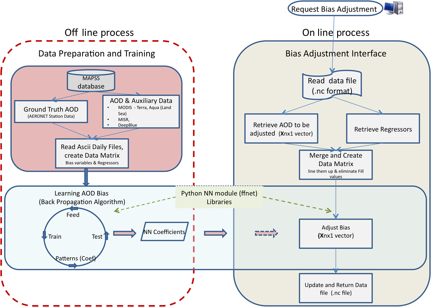 Component A of the offline process is the training data set preparation from the MAPSS data base. In this step, data are retrieved from original MAPSS ASCII files with corresponding regressors, creating information matrices with time labels and location information. Then the data are transformed to a shape where the NN module can accept for further process. Finally, the prepared matrices are saved for later use. Component B is the training process. The shaped data from step A is randomly separated into 90% training and 10% testing blocks. Training data is processed using Feed-Forward Neural Network for Python (FFNET) software28 with a given number of nodes and hidden layers. The overall NN algorithm can be described as the following: (1) network architecture: feed-forward (no cycles); (2) optimization algorithm: back propagation; (3) hidden layers: one; and (4) nodes: 60 to 100 depending on the data set in consideration (land, ocean). In order to use the data set properly, all the regressors (i.e., auxiliary data) have to be present at a specific data point that needs to be adjusted. If this is not the case, then that data point is dropped. Finally, the NN coefficients are obtained from the 90% training blocks and are saved for comparison and utilization by the online process. The 10% testing blocks are used to evaluate the NN performance (over fitting, etc.). Table 2 lists the details of data volumes for training and testing before and after data elimination. Table 2Number of data points after separating each case, ocean and land, and filtering out as defined below. To use each data point in neural network (NN) training, it is a requirement to have all the regressors present. If a data point cannot satisfy this requirement, it is dropped and called stage 1 filtering.
In this work, the NN is also implemented within the framework of the Giovanni system29,30 to provide on-the-fly bias estimation/adjustment ( http://giovanni.gsfc.nasa.gov/aerostat/) using trained data coefficients (provided from the offline phase). The schematic diagram is shown in the right panel of Fig. 3. There are three main components for the online phase:
Calculation of adjusted AOD values: the created matrices are sent to the module to obtain bias adjusted AOD values. Adjusted AOD are appended to the same data files and returned. One important issue for NN training is the selection of the regressors. We understand that the selection of regressors is not a straightforward process because of the dynamically changing characteristics of atmospheric variables and it requires special attention. We use expert opinions to design a brute force approach where multiple NN experiments are performed for different settings of regressors and compared to GT data. For training purposes, the best combinations of regressors resulting from our trials are considered. 5.Experiments and ResultsWe evaluated the NN adjustment on four AOD retrieval cases: MODIS-Terra Land, MODIS-Terra Ocean, MODIS-Aqua Land, and MODIS-Aqua Ocean, globally collocated with AERONET AOD in time and space. The first step in investigating the relationship between any two independent variables is to put the two variables on the scatter plot. For example, Figs. 4(a) and 4(b) represent the scatter plot for MODIS-Aqua Ocean AOD, and Figs. 4(c) and 4(d) represent the Land AOD with respect to collocated AERONET AOD. Additional statistical measures [ (red line), linear regression (black line), the expected error (EE) bounds (red dotted lines), and data number density distribution (color contours)] are also provided. The EE bounds contain the mean and first standard deviation (66%) of all points. Levy et al.31 defined the EE bounds for the MODIS Land case expressed in Eq. (8) and for the MODIS Ocean case expressed in Eq. (9) and where is AOD at 550 nm. In general, the larger the number of estimated AOD data within the EE cone/envelope, the better the results are. Because of the high number of data, there is a significant overlap among data points. Under these conditions, the scatter plots become less informative for observing the relationships. Therefore, additional data number density distributions (kernel density estimates) are overplotted to show the majority of the data points appearing for small AOD values () and fewer data points appearing for larger AOD values.Fig. 4Scatter plots for MODIS-Aqua Aerosol Optical Depth at 550 nm where the first row is the ocean, and the second is the land. The -axis of each plot is the AERONET AOD and -axis is the MODIS data. (a and c) before NN adjustment; (b and d) after NN adjustment.  The statistical measures of the four cases with NN adjustments are summarized in Table 3, which also includes a comparison of the values obtained before and after applying the NN adjustments. Overall, there is an improvement for all cases after applying NN adjustments, including root mean square error reduction, increased correlation coefficients between the estimates and GT, and the increased percentage of data within the EE error cone. However, notice that the linear regression line for the adjusted MODIS AOD moved away from the 1:1 line, as compared to the linear regression line for the original MODIS AOD. In combining with number density contours, the different tendencies on the scatter plot can be seen for smaller AOD values compared to the higher values. It should also be noted that high AOD values affect the regression slope, while the majority of measurements are within the low AOD. Also the variance of the MODIS AOD data on the global scale is much larger compared to the variance of the bias-adjusted AOD estimations. It should be noted that the NN-estimated AOD values are slightly smaller than reference AERONET AOD in contrast to the higher retrieved MODIS AOD. These results are reported from the training data set. For the testing data, the results have similar or slightly lesser performance, as expected. An example run for testing is summarized in Table 3. Table 3Summary of the improvements from original data to NN approximation (A) Training (B) Testing.
To better evaluate the impact from NN-adjusted AOD, we can compare Figs. 1(a) to 5(a), which overlays additional information from NN-adjusted AOD for MODIS-Aqua Land. The improvements are obtained for most AOD bins when comparing NN estimates versus the original MODIS data. As shown in Fig. 5(a), the variances in NN-adjusted AOD are smaller than those of the original data sets. However, it should be noted that during extreme events such as fires or volcanic eruptions, higher spreads with AOD retrieved values could be expected, causing larger variances for both the adjusted and unadjusted data. In any case, the NN-adjusted variances still remain smaller than unadjusted ones. In terms of outliers, the NN-estimated values for the outliers move closer to the AERONET in the AOD range between 0 and 1. Most of the outliers are smoothed out. Figure 5(b) shows that the normality of the residuals has been improved after the NN adjustment. The improvements for other cases, including MODIS-Aqua Ocean, MODIS-Terra Land, and MODIS-Terra Ocean, have shown similar results and thus are not discussed here. Fig. 5(a) MODIS-Aqua Land box plot for each bin with interval of 0.03. Black boxes are AERONET, red boxes are the original AOD data, and blue boxes are the NN estimates. (b) Q-Q plots at 550 nm, at the right of each group (i) MODIS-Aqua Land versus AERONET, (ii) MODIS-Aqua Land residuals (AERONET minus the corresponding MODIS). Here, the -axis is the sample quantile, and the -axis is the theoretical quantile.  Since NN does its job on the basis of the given training data (whether correct or not), in order to solve the problem of the large spread, extreme cases must be studied further, and new feature vectors should be added to the training data that could better represent such events. Another important factor that needs to be considered is the local effect. For example, Fig. 6 scatter plots show unadjusted (right) and adjusted (left) AOD over the Mauna Loa station from both AERONET and collocated MODIS-Aqua AOD. It can be observed that only 9.2% of the data is within the EE range before the adjustment, and after the adjustment, this amount increases to 38%. Although this seems a good improvement, we still need to understand the reasons for the existence of the higher variance MODIS data and much higher MODIS-Aqua estimated values compared to the AERONET station data. The analysis from Ristovski et al.16 revealed that the Mauna Loa (Hawaii) and the Izana (Spain) sites are located at high elevations and the behavior of the data is very different from other AERONET sites. This implies an extension of this work from global to regional cases in terms of data collection and reanalysis. 6.SummaryIn this study, we have shown the success and some of the benefits of the bias adjustment on MODIS AOD at 550 nm for both the Aqua and Terra MODIS instrument, using a nonparametric NN method with one hidden layer. The biases for the MODIS retrieved AOD were based on the quality-assured coincident AOD data from 537 AERONET stations. Because of the global nature of the data set, the bias removal or improvements are considered in a global sense only. Therefore, the global improvements do not necessary reflect the degree of improvement in local or regional results for every particular station. The test results showed that in most of the stations the bias-adjusted AOD was closer to the corresponding AERONET AOD but did not perform uniformly well across all the stations. It should be noted that NN can only be as successful as the provided data set. This implies that NN can be as good as the aerosol retrieval algorithm provided feature vectors. For example, if an algorithm is not able to capture extreme events, that means feature vectors that are representing such an event will not be represented in the training data set. This suggests that there is room for further improvement by adding regional studies such as Mauna Loa and Izana and extreme events as feature vectors in the training data sets. Another shortcoming is the number of data that are considered for the oceans. It is well known that there are not enough AERONET stations over open oceans. It is highly expected that including data gathered from ship measurements (such as Marine Aerosol Network) will increase the tractability of the estimations. In addition, the AERONET data are accepted as GT in this study; however, it should be noted that AERONET has its own uncertainties. Furthermore, additional information such as cross satellite information, surface albedo, surface wind, etc., can be included in the regressors for further improvement of the results. Finally, we used one hidden layer, a nonlinear activation function, and a sufficient number of hidden neurons for the NN architecture. In summary, the advantages of the NN approach are fourfold:12,32,33
There are still some potential disadvantages to the NN approach, as described below.
Despite the potential shortcomings in the study we have demonstrated that the NN strategy offers significant improvement to global estimates of AOD from MODIS and other instruments. Such improvements can translate to overall accuracy improvement for global radiation budgets. AcknowledgmentsSupport for the development of this online platform for statistical intercomparison of aerosols has been provided by NASA HQ (PM: Stephen Berrick) through the ROSES 2009 ACCESS Program (PI: Gregory Leptoukh). We thank the science and support teams of MODIS and AERONET for their data. We also thank the principal investigators (PIs) of AERONET sites and their supporting staff for making data available. We especially would like to dedicate the paper to the PI for this project, Dr. Gregory Leptoukh, who suddenly passed away before the project completion. This work would not have been possible without Dr. Leptoukh’s great vision, support, and guidance. Finally, we would like to express our appreciation to Dr. Jim Acker for his valuable comments and editing. ReferencesZ. Liet al.,
“Uncertainties in satellite remote sensing of aerosols and impact on monitoring its long-term trend: a review and perspective,”
Ann. Geophys., 27
(7), 2755
–2770
(2009). http://dx.doi.org/10.5194/angeo-27-2755-2009 1593-5213 Google Scholar
L. A. Remeret al.,
“The MODIS aerosol algorithm, products, and validation,”
J. Atmos. Sci., 62
(4), 947
–973
(2005). http://dx.doi.org/10.1175/JAS3385.1 JAHSAK 0022-4928 Google Scholar
R. Kahnet al.,
“Satellite-derived aerosol optical depth over dark water from MISR and MODIS: comparisons with AERONET and implications for climatological studies,”
J. Geophys. Res., 112
(D18), D18205
(2007). http://dx.doi.org/10.1029/2006JD008175 JGREA2 0148-0227 Google Scholar
R. C. Levyet al.,
“Global evaluation of the collection 5 MODIS dark-target aerosol products over land,”
Atmos. Chem. Phys. Discuss., 10 14815
–14873
(2010). http://dx.doi.org/10.5194/acpd-10-14815-2010 1680-7367 Google Scholar
T. X. P. Zhaoet al.,
“Study of long-term trend in aerosol optical thickness observed from operational AVHRR satellite instrument,”
J. Geophys. Res., 113
(D7), 1
–14
(2008). http://dx.doi.org/10.1029/2007JD009061 JGREA2 0148-0227 Google Scholar
A. Ignatovet al.,
“Two MODIS aerosol products over ocean on the terra and aqua CERES SSF datasets,”
J. Atmos. Sci., 62
(4), 1008
–1031
(2005). http://dx.doi.org/10.1175/JAS3383.1 JAHSAK 0022-4928 Google Scholar
T. L. Andersonet al.,
“Mesoscale variations of tropospheric aerosols,”
J. Atmos. Sci., 60
(1), 191
–136
(2003). http://dx.doi.org/10.1175/1520-0469(2003)060%3C0119:MVOTA%3E2.0.CO;2 Google Scholar
N. G. Loebet al.,
“Fusion of CERES, MISR, and MODIS measurements for top-of-atmosphere radiative flux validation,”
J. Atmos. Sci., 111
(D18), D18209
(2006). http://dx.doi.org/10.1029/2006JD007146 JAHSAK 0022-4928 Google Scholar
A. A. Kokhanovskyet al.,
“Aerosol remote sensing over land: a comparison of satellite retrievals using different algorithms and sensors,”
Atmos. Res., 85
(3–4), 372
–394
(2007). http://dx.doi.org/10.1016/j.atmosres.2007.02.008 ATREEW 0169-8095 Google Scholar
J. ZhangJ. S. Reid,
“MODIS aerosol product analysis for data assimilation: assessment of over-ocean level 2 aerosol optical thickness retrievals,”
J. Geophys. Res., 111
(D22), D22207
(2006). http://dx.doi.org/10.1029/2005JD006898 JGREA2 0148-0227 Google Scholar
S. M. Kinneet al.,
“An aerocom initial assessment optical properties in aerosol component modules of global models,”
Atmos. Chem. Phys., 6
(7), 1815
–1834
(2006). http://dx.doi.org/10.5194/acp-6-1815-2006 ACPTCE 1680-7316 Google Scholar
C. M. Bishop, Neural Networks for Pattern Recognition, Clarendon Press, Oxford
(1995). Google Scholar
M. T. HaganH. B. DemuthM. Beale, Neural Network Design, PWS Publishing Co, Boston
(1996). Google Scholar
S. Lianget al.,
“Estimation and validation of land surface broadband albedos and leaf area index from EO-1 ALI data,”
IEEE Trans. Geosci. Rem. Sens., 41
(6), 1260
–1267
(2003). IGRSD2 0196-2892 Google Scholar
R. V. Leslieet al.,
“Neural network microwave precipitation retrievals and modeling results,”
Proc. SPIE, 7154 715406
(2008). http://dx.doi.org/10.1117/12.804815 PSISDG 0277-786X Google Scholar
K. Ristovskiet al.,
“Uncertainty analysis of neural-network-based aerosol retrieval,”
IEEE Trans. Geosci. Rem. Sens., 50
(2), 409
–414
(2012). http://dx.doi.org/10.1109/TGRS.2011.2166120 IGRSD2 0196-2892 Google Scholar
D. Daset al.,
“Reducing need for collocated ground and satellite based observations in statistical aerosol optical depth estimation,”
in IEEE International Int. Geosci. Remote Sens. Symposium,
II-879
–II-882
(2008). Google Scholar
B. HanZ. L. Z. ObradovicS. Vucetic,
“A statistical complement to deterministic algorithms for retrieving aerosol optical thickness from radiance data,”
Eng. Appl. Artif. Intell., 19
(7), 787
–795
(2006). http://dx.doi.org/10.1016/j.engappai.2006.05.009 Google Scholar
A. Cazorlaet al.,
“Technical note: determination of aerosol optical properties by a calibrated sky imager,”
Atmos. Chem. Phys., 9
(17), 6417
–6427
(2009). http://dx.doi.org/10.5194/acp-9-6417-2009 ACPTCE 1680-7316 Google Scholar
D. J. Laryet al.,
“Machine learning and bias correction of MODIS aerosol optical depth,”
IEEE Trans. Geosci. Rem. Sens., 6
(4), 694
–698
(2009). http://dx.doi.org/10.1109/LGRS.2009.2023605 IGRSD2 0196-2892 Google Scholar
A. Smirnovet al.,
“Cloud screening and quality control algorithms for the AERONET database,”
Remote Sens. Environ., 73
(3), 337
–349
(2000). http://dx.doi.org/10.1016/S0034-4257(00)00109-7 RSEEA7 0034-4257 Google Scholar
B. N. Holbenet al.,
“AERONET—a federated instrument network and data archive for aerosol characterization,”
Rem. Sens. Environ., 66
(1), 1
–16
(1998). http://dx.doi.org/10.1016/S0034-4257(98)00031-5 RSEEA7 0034-4257 Google Scholar
C. Ichokuet al.,
“A spatio-temporal approach for global validation and analysis of MODIS aerosol products,”
Geophys. Res. Lett., 29
(12), 1008
–1031
(2002). http://dx.doi.org/10.1029/2001GL013206 GPRLAJ 0094-8276 Google Scholar
M. PetrenkoC. IchokuG. Leptoukh,
“Multi-sensor aerosol products sampling system (MAPSS),”
Atmos. Meas. Tech., 5
(1), 913
–926
(2012). http://dx.doi.org/10.5194/amt-5-913-2012 AMTTC2 1867-1381 Google Scholar
R. C. Levyet al.,
“Algorithm for remote sensing of tropospheric aerosol over dark targets from MODIS,”
(2009). Google Scholar
R. A. Kahnet al.,
“MISR aerosol product attributes, and statistical comparisons with MODIS,”
IEEE Trans. Geosci. Rem. Sens., 47
(12), 4095
–4114
(2009). http://dx.doi.org/10.1109/TGRS.2009.2023115 IGRSD2 0196-2892 Google Scholar
T. F. Ecket al.,
“Wavelength dependence of the optical depth of biomass burning, urban, and desert dust aerosols,”
J. Geophys. Res., 104
(D24), 31333
–31349
(1999). http://dx.doi.org/10.1029/1999JD900923 JGREA2 0148-0227 Google Scholar
M. Wojciechowski, Feed-Forward Neural Network for Python, Poland
(2011). Google Scholar
J. AckerG. Leptoukh,
“Online analysis enhances use of NASA Earth science data,”
EOS Trans. Amer. Geophysical Union, 88
(2), 14
–17
(2007). Google Scholar
S. Berricket al.,
“Giovanni: a web services workflow-based data visualization and analysis system,”
IEEE Trans. Geosci. Rem. Sens., 47
(1), 106
–113
(2009). http://dx.doi.org/10.1109/TGRS.2008.2003183 Google Scholar
M. C. Levyet al.,
“Evaluation of the MODIS aerosol retrievals over ocean and land during clams,”
J. Atmos. Sci., 62
(4), 974
–992
(2005). http://dx.doi.org/10.1175/JAS3391.1 JAHSAK 0022-4928 Google Scholar
R. J. Boik, Classical Multivariate Analysis, Lecture Notes, Department of Mathematical Sciences, Montana State University Bozeman(2004). Google Scholar
A. Iscanoglu, Credit Scoring Methods and Accuracy Ratio, Middle East Technical University,
(2005). Google Scholar
Biography Arif Albayrak received his BS degree in mathematical engineering from Yildiz Technical University, and the MS degree in mathematics from California State Polytechnic University. He specializes in estimation and prediction techniques and learning algorithms. He is currently employed as a scientist/algorithm developer with ADNET Systems, Inc., and working at the NASA Goddard Space Flight Center, Greenbelt, MD.  Jennifer Wei received her BA degree in atmospheric science from National Taiwan University, Taiwan, in 1992, the MS degree in environmental science from New Jersey Institute of Technology, Newark, in 1995, and the PhD degree in atmospheric science from the University of Illinois at Urbana-Champaign in 2002. She is currently a principle support scientist with ADNET Systems, Inc., Rockville, MD, working at the NASA Goddard Space Flight Center, Greenbelt, MD. Her research interests include remote sensing data processing, retrieval algorithms, and visualization of large earth science data sets. She is currently involved to develop algorithms and programs used for the analysis and processing of related data and contribute to multi-sensor and model data analysis and online analysis system development.  Maksym Petrenko is a research associate for Earth System Science Interdisciplinary Center (ESSIC) on-site at the NASA Goddard Space Flight Center, Climate and Radiation Branch. Maksym joined ESSIC in 2009 after a PhD in computer science from Wayne State University, Detroit. His BS (2003) and MS (2005) degrees are also in computer science and were received from the National University of Kiev-Mohyla Academy, Kiev, Ukraine. In his PhD studies and prior projects, he focused on data analysis and effective ways for expanding complex software systems with new features. With this experience, he joined Dr. Charles Ichoku at NASA to work on the Mutli-sensor Aerosol Products Sampling System (MAPPS) that seeks to provide an approach and a unified framework for inter-comparison and validation of aerosol measurements from different sensors and instruments, including ground-based, airborne, and spaceborne, obtained at different locations and time around the globe.  Christopher Lynnes received his BA degree in earth sciences from Dartmouth College in 1981, and the MS and PhD degrees in geophysics from the University of Michigan in 1984 and 1988, respectively. He is the chief systems engineer for the Goddard Earth Sciences Data and Information Services Center.  Robert C. Levy received the BA, MS, and PhD degrees from Oberlin College (1994), Colorado State University (1996), and the University of Maryland—College Park (2007), respectively. He joined SSAI as a member of the MODIS aerosol team in 1998, and is responsible for upkeep, validation and improvement of the MODIS aerosol retrieval algorithms. Along with developing a highly useful and successful product, he has collaborated with research groups around the world. His research has ranged from applications of new algorithm development, monitoring surface air quality, aerosol/cloud interactions and aerosol trends. In 2012, he was the recipient of the Young Scientist award from the International Radiation Commission. |
|||||||||||||||||||||||||||||||||||||||||||||||||||||||||||||||||||||||||||||||


