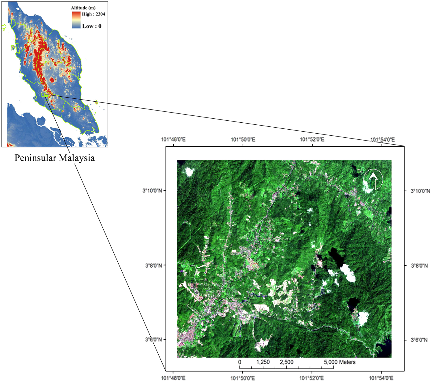
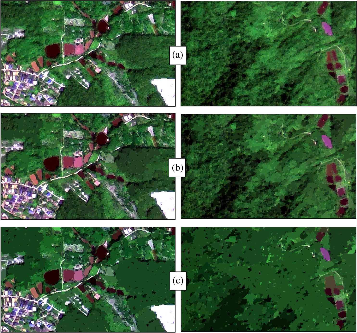
1.

Introduction

Decision making in each country or region needs adequate information on many complex interrelated aspects of its activities. Land use is desired as one such aspect and necessary knowledge about land use and land cover has become increasingly important.¹ Classification of land use and land cover based on remotely sensed imagery can be partitioned into two general image analysis methods. The first approach is based on pixels, which has long been employed for classifying remotely sensed imagery. The second approach is based on objects, which has become increasingly common over the last decade.^2,3

The conventional pixel-based classification techniques, such as maximum likelihood classifier (MLC), have been extensively used for the extraction of thematic information since the 1980s.^4,5 MLC, the most established approach of image classification,^6,7 assumes a normal Gaussian distribution of multivariate data. In this method, pixels are allocated to the most likely output class or allocated to a class based on a posterior probability of membership and dimensions equal to the number of bands in the original image.⁸ This requires users to carefully determine the classification scheme, so that each class follows a Gaussian distribution, and MLC ideally has to be performed at the spectral class level.⁷ Some examples of MLC application for land use and land cover classification include comparison of MLC and artificial neural network in USA using Landsat Thematic Mapper (TM) data,⁹ the same comparison in Turkey using Landsat TM data,¹⁰ an evaluation of fuzzy classifier and MLC using Landsat Enhanced ${\mathrm{TM}}^{+}$ (${\mathrm{ETM}}^{+}$) data in Iran,¹¹ and a comparison between object-oriented classification and MLC using Advanced Spaceborne Thermal Emission and Reflection Radiometer (ASTER) data in China.¹²

In terms of classification results, MLC is more suitable for remote-sensing imagery with medium and low spatial resolution, but it cannot exploit the full advantages of ground geometric structure and texture information contained in high-spatial-resolution imagery.¹² The object-oriented classification method relies on the spectral characteristics of ground and makes further use of geometric and structural information.^12,13 In this method, an object is a region of interest with spatial, spectral (brightness and color), and/or textural characteristics that define the region.¹⁴ Several studies have been conducted to compare object-based classification method with pixel-based techniques. For example, Yan et al.¹³ compared MLC with a $K$-nearest neighbor ($K$-NN) object-based analysis using ASTER imagery. They indicated that the overall accuracy of the object-based $K$-NN classification considerably outperformed the pixel-based MLC classification in Wuda, China (83.25% and 46.48%, respectively). A comparison between MLC and $K$-NN object-based classification method was performed using a decision tree approach based on high-spatial resolution digital airborne imagery.¹⁵ This study in northern California showed that $K$-NN object-based classification with one nearest neighbor (NN) gave a higher performance than MLC by 17%. Another comparison in Gettysburg, Pennsylvania, between MLC and $K$-NN object-based classifier was carried out by Platt and Rapoza¹⁶ using multispectral IKONOS imagery. They revealed that using expert knowledge the object-based $K$-NN classifier had the best overall accuracy of 78%. The application of object-based classifier using pan-sharpened Quickbird imagery in agricultural environments led to a higher accuracy (93.69%) than MLC application (89.6%) in southern Spain.¹⁷ Myint et al.¹⁸ used Quickbird imagery to classify urban land cover in Phoenix, Arizona. They compared MLC with a $K$-NN object-based classifier and concluded that object-based classifier with an overall accuracy of 90.4% outperformed MLC with an overall accuracy of 67.6%. In another study, application of object-based classifier on Système Pour l’Observation de la Terre (SPOT)-5 Panchromatic (PAN) imagery demonstrated more feasibility in the study site (Beijing Olympic Games Cottage) than conventional pixel-based approaches.⁵

The use of kappa index agreement¹⁹ along with “proportion correct” has become customary in remote-sensing literature for the purpose of accuracy assessment. Pontius²⁰ and Pontius and Millones²¹ exposed some of the conceptual problems with the standard kappa and proposed a suite of variations on kappa to remedy the flaws of the standard kappa. Typically, the kappa statistic compares accuracy with a random baseline. According to Pontius and Millones,²¹ however, randomness is not a logical option for mapping. In addition, several kappa indices suffer from basic theoretical errors. Therefore, the standard kappa and its variants are more often than not complicated for computation, difficult to understand, and unhelpful to interpret.^22,21 As such, in this study, two components of disagreement between classified and ground-truthed maps, in terms of the quantity and spatial allocation of the categories as suggested by Pontius and Millones,²¹ were employed.

This work was aimed at evaluating the capability of MLC and $K$-NN object-based classifier for land-use classification of the Langat basin that was captured on a SPOT-5 imagery.

2.

Materials and Methods

2.1.

Study Area

The Langat basin is located at the southern part of Klang Valley, which is the most urbanized river basin in Malaysia. In recent decades, the Langat basin has undergone rapid urbanization, industrialization, and agricultural development.²³ The Langat basin is also a main source of drinking water for the surrounding areas, is a source of hydropower, and plays an important role in flood mitigation. Over the past four decades, the Langat basin has served 50% of the Selangor State population. Its average annual rainfall is 2400 mm. The basin has a rich diversity of landforms, surface features, and land cover.^24,25

Due to the national importance of the Langat basin, a pilot region (upstream of the Langat river) with a total area of $111.17{\mathrm{k}\mathrm{m}}^2$ was selected for land-use classification using a SPOT-5 imagery (Fig. 1).

Fig. 1

Study area represented by a false-color composite.

2.4.

Image Segmentation

Segmentation, a fundamental first step in object-based image analysis,³ is the process of partitioning an image into segments by grouping neighboring pixels with similar feature values such as brightness, texture, and color. These segments ideally correspond to real-world objects.¹⁴ Environment for Visualizing Images EX employs an edge-based segmentation algorithm that is very fast and requires only one input parameter [scale level (SL)]. By suppressing weak edges to different levels, the algorithm can yield multiscale segmentation results from finer to coarser segmentation.¹⁴ The selection of an appropriate value for the SL is considered as the most important stage in object-based image analysis.³ SL is a measure of the greatest heterogeneity change when the two objects are merged, which is used as a threshold after calculation to terminate segmentation arithmetic.^31,5 This value controls the relative size of the image objects, which has a direct impact on the classification accuracy of the final map.^3,18 Generally, choosing a high SL causes fewer segments to be defined and choosing a low SL causes more segments to be defined.¹⁴ In this study, based on previous experiences and literature recommendations,^32,5,15 three levels of scale factor, i.e., 10, 30, and 50, were used in image segmentation (Fig. 2).

Fig. 2

Image segmentation using different scale levels: (a) $\mathrm{SL}=10$, (b) $\mathrm{SL}=30$, and (c) $\mathrm{SL}=50$.

2.6.

Accuracy Assessment

Ground-truth map was prepared based on the observed data (2006 land-use map) and field survey in about 10% of the total area. Disagreement parameters determine the disagreement between simulated and observed maps.^22,21,35,36 Quantification error [quantity disagreement (QD)] happens when the quantity of cells of a category in the simulated map is different from the quantity of cells of the same category in the reference map. Location error [allocation disagreement (AD)] occurs when location of a class in the simulated map is different from location of that class in the reference map.²¹

2.6.1.

Disagreement Components

Table 1

Format of estimated population matrix (adapted from Ref. 21).

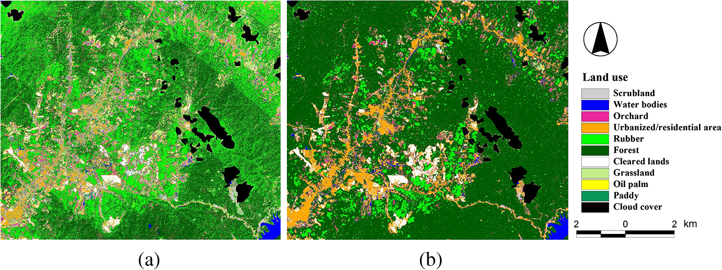
In reference to Table 1, $J$ refers to the number of categories and number of strata in a typical stratified sampling design. Each category in the comparison map is indexed by $i$, which ranges from 1 to $J$. The number of pixels in each stratum is denoted by $N_i$. Each observation is recorded based on its category in the comparison map ($i$) and the reference map ($j$). The number of these observations is summed as the entry $n_{ij}$ in row $i$ and column $j$ of the contingency matrix. Proportion of the study area ($P_{ij}$), i.e., category $i$ in the simulated map and category $j$ in the observed map, is estimated by the following equation^22,21:

Eq. (2)

$$p_{ij}=\left(\frac{n_{ij}}{{\sum }_{j=1}^J{n}_{ij}}\right)\left(\frac{N_i}{{\sum }_{i=1}^J{N}_i}\right).$$

QD ($q_g$) for an arbitrary category $g$ is calculated as follows:

Eq. (3)

$$q_g=\left|\right(\sum _{i=1}^J{p}_{ig})-(\sum _{j=1}^J{p}_{gj}\left)\right|.$$

Overall QD, which incorporates all $J$ categories, is calculated as follows:

Eq. (4)

$$\mathrm{QD}=\frac{{\sum }_{g=1}^J{q}_g}{2}.$$

Calculation of AD ($a_g$) for an arbitrary category $g$ is shown in Eq. (5). The first argument within minimum function is the omission of category $g$, while the second argument is the commission of category $g$.

Eq. (5)

$$a_g=2\min \left[\right(\sum _{i=1}^J{p}_{ig})-p_{g{g}^{\prime }}(\sum _{j=1}^J{p}_{gj})-p_{gg}].$$

Overall AD is calculated as follows:

Eq. (6)

$$\mathrm{AD}=\frac{{\sum }_{g=1}^J{a}_g}{2}.$$

Proportion of agreement ($C$) is calculated as follows:

Eq. (7)

$$C=\sum _{j=1}^J{p}_{jj}.$$

Total disagreement ($D$), the sum of overall quantity of disagreement and overall allocation of disagreement, is computed as follows:

Eq. (8)

$$D=1-C=\mathrm{QD}+\mathrm{AD}.$$

3.

Results and Discussion

Figure 3 illustrates the maps classified using MLC and SL30-NN5 (object-based classifier). Table 2 gives the disagreement components, calculated for each land-use category and the total landscape, based on MLC and object-based classification. QD and AD in the total landscape using MLC were 11.66% and 22.38%, respectively. In comparison with object-based image classifiers, MLC resulted in the lowest QD. Nevertheless, due to its highest AD, MLC resulted in a higher total disagreement in the total landscape. The ratio of QD to areal proportion (AP) and AD to AP of each land-use category gives a better inference about the contribution of each land acreage unit toward error production. From Table 2, paddy, oil palm, and grassland yielded the highest QD/AP using ML classifier, which indicates the lowest accuracy in terms of quantity of classified pixels. Scrubland, orchard, and oil palm yielded the highest AD/AP, which indicates the lowest accuracy in terms of location of the classified pixels. Among paired land-use categories, orchard/oil palm showed the lowest spectral separability with a Jeffries–Matusita distance of 0.1. As such, it would be challenging to discriminate between orchard and oil palm stands using MLC. The spectral separability between scrubland and paddy was also comparatively low, i.e., 0.7. Paired land-use categories with low spectral separability can be expected to demonstrate higher QDs and ADs.

Fig. 3

Maps classified using (a) maximum likelihood classifier (MLC) and (b) SL30-NN5.

Table 2

Accuracy assessments of different land-use categories derived using maximum likelihood classifier (MLC) and object-based classification.

Among the object-based image classifiers, SL30-NN5 showed the highest accuracy with a QD of 15% and an AD of 6.33% in the total landscape (Table 2). Using SL30-NN5, oil palm, paddy, and scrubland yielded the highest QD/AP, i.e., 0.8%, 0.77%, and 0.72%, respectively. Orchard and grassland with an AD/AP of 0.76% and 0.44%, respectively, yielded the highest allocation error.

SL30-NN5 resulted in spatial and/or spectral similarity on the image, which exerted some difficulty in accurately discriminating between rubber and forest, orchard and oil palm, and paddy and scrubland (Table 3). These results are supported by the Jeffries–Matusita distance values (Fig. 4). As indicated in Table 2, SL30-NN5 reduced allocation error by 250% as compared with MLC. However, MLC showed 22% improvement in quantity accuracy as compared to SL30-NN5.

Table 3

Spatial, spectral, and textural properties used in object-based image classification (extracted from the SL30-NN5-classified image).

Fig. 4

Pair separation based on the Jeffries–Matusita distance.

Results suggest that object-based classification, in comparison with pixel-based classification, offered a more realistic and accurate land-use map. This finding is in conformity with previous reports documented by Wang et al.,⁵ Yan et al.,¹³ Chen et al.,³⁷ Gao et al.,³⁸ and Myint et al.¹⁸

Despite the higher capability of object-oriented approach in image classification, differences in execution time between pixel- and object-based image analysis still remain an issue, especially for large areas.³ Future development of more quantitative methods for selecting optimal image segmentation parameters, especially at the SL as demonstrated by Costa et al.³⁹ and Drăgut et al.,⁴⁰ will hopefully reduce the required time for object-oriented classification.³

This work demonstrated the utility of disagreement components in validating land-use classification approaches, which has been confirmed by Memarian et al.²² and Pontius and Millones.²¹

Based on the results obtained in this study and previous investigations on object-based image classification reported by Yu et al.,¹⁵ Platt and Rapoza,¹⁶ and Duro et al.,³ the following refinements are recommended for future work in obtaining a more precise land-use map:

4.

Conclusion

In comparison with object-based image classification, the MLC resulted in a higher total disagreement in total landscape. Image classification employing the MLC yielded a high ratio of QD to AP in land-use categories such as paddy, oil palm, and grassland and consequently low accuracy in terms of quantity of classified pixels. Meanwhile, categories such as scrubland, orchard, and oil palm, which showed a high ratio of AD to AP, registered low accuracy in terms of location of classified pixels. These results were supported by low separation distance between paired classes. Object-based image classifier with the SL of 30 and the $K$-value of 5 (SL30-NN5) showed the highest classification accuracy. Using the SL30-NN5, oil palm, paddy, and scrubland yielded high QD/AP values, while orchard and grassland showed the highest allocation error. Nevertheless, SL30-NN5 resulted in spatial and/or spectral similarity that caused difficulty in discriminating between rubber and forest, orchard and oil palm, and paddy and scrubland. Evidently, SL30-NN5 reduced allocation error by 250% as compared with MLC. However, MLC showed 22% improvement in quantity accuracy as compared with SL30-NN5.

This work has demonstrated higher performance and utility of object-based classification over the traditional pixel-based classification in a tropical landscape, i.e., Malaysia’s Langat basin.