Recognition and characterization of migratory movements of Australian plague locusts, Chortoicetes terminifera, with an insect monitoring radar

V. Alistair Drake; Haikou Wang

doi:10.1117/1.JRS.7.075095

5 September 2013 Recognition and characterization of migratory movements of Australian plague locusts, Chortoicetes terminifera, with an insect monitoring radar

V. Alistair Drake, Haikou Wang

Author Affiliations +

Journal of Applied Remote Sensing, Vol. 7, Issue 1, 075095 (September 2013). https://doi.org/10.1117/1.JRS.7.075095

Abstract

Two special purpose insect-detecting radar units have operated in inland eastern Australia, in the region where nocturnal migratory movements of Australian plague locusts Chortoicetes terminifera occur, for over 10 years. The fully automatic radars detect individual insects as they fly directly overhead and “interrogate” them to obtain information about their characters (size, shape, and wing beating) and trajectory (speed, direction, and orientation). The character data allow locusts to be distinguished from most other migrant species. A locust index, calculated from the total count of locust-like targets for a night, provides a simple indication of migration intensity. For nights of heavy migration, the variation of numbers, directions, and speeds with both height and time can be examined. Emigration and immigration events can be distinguished, as can “transmigration,” the passage overhead of populations originating elsewhere. Movement distances can be inferred, and broad source and (more tentatively) destination regions are identified. Movements were typically over distances of up to 400 km. Interpretation of radar observations requires judgment, and the present two units provide only partial coverage of the locust infestation area, but their capacity to detect major population movements promptly, and to provide information between necessarily infrequent surveys, has proved valuable.

1. Introduction

The Australian plague locust, Chortoicetes terminifera, an acridid grasshopper, is an important migratory pest of agricultural crops and pasture in both eastern and western Australia.¹^,² Populations develop in inland pastures following rain and the adults undertake postfledging night flights over distances of up to a few hundred kilometers. These migrations, and subsequent daytime redistribution flights over distances of tens of kilometers, can carry populations into areas where they can cause significant economic damage,³ both directly and by initiating a subsequent “hopper” (nymphal) infestation. In eastern Australia, movements tend to be northward in spring, out of temperate-zone regions with winter rainfall, and southward in autumn out of the adjacent subtropical summer-rainfall zone.¹^,⁴ Populations in the subtropical rangelands of southeastern Queensland can grow rapidly in years with high summer rainfall, and this area is often regarded as the source of major outbreaks and plagues.⁵ The main management strategy for this species is pre-emptive control in the inland, with the aim of suppressing, or at least reducing, population build-up before the locusts move southwards or eastwards into the cropping belt.⁶^–⁸

Entomological radars have been used to study insect migration in Australia since the 1970s, and C. terminifera has been the species under observation on a number of occasions.⁹^,¹⁰ Locusts are well suited to radar observation, as their relatively large size makes them easy to detect and they are often so numerous that there is little doubt about the identity of the targets the radar is detecting. Since 1999, two insect monitoring radars (IMRs)¹¹ have been deployed, $\sim 300 km$ apart, in inland eastern Australia within the broad region where C. terminifera populations develop and strategic control occurs.¹² These radars, which operate at an X-band frequency (9.4 GHz, wavelength 32 mm), are fully automated and operated for 11 h each night. The observations, which are available the next morning via a telephone link, are used operationally by the Australian Plague Locust Commission (APLC) as a supplementary source of information, specifically on movements of adult populations. They are also incorporated into a multiple-year accumulating dataset that forms the basis for analyses of movement patterns, of seasonal and year-to-year variations, and of correlations with environmental variables.⁴^,¹⁰

The type of information about locust populations that a radar provides differs in several ways from that available from more conventional sources. In particular, the insects being observed are inaccessible—they can be over 1 km above the surface—and thus no specimens are available to confirm their identity. Therefore, at least in the case of routine, fully automated observations, the type of target being observed—whether they are locusts or some other insect species, or even bats or birds—must be inferred from the radar signal itself. (Precipitation echo must also be eliminated though its different form makes this relatively straightforward.) In the first part of this article, the characters that are used to discriminate echo signals from locusts will be described. When the radar shows locust echoes to be numerous, either throughout or for part of a night, estimates can be made of the intensity of the movement, its direction, the distance covered, and whether the source and destination regions were nearby or a few hundred kilometers away, all of which are of obvious potential value for locust monitoring and planning of ground or aerial surveys. The second part of the article will present some radar observations of locust movements and indicate how they can be interpreted to provide the information about spatial population processes that locust managers need, both for operational decision making and to recognize patterns of outbreak development and persistence. All data presented in this article are from the IMR at Bourke airport (30°2′ S, 145°57′ E) in northwestern New South Wales, Australia, and were obtained during the 2007 to 2008 insect-flight season.

2. Insect Monitoring Radars

IMRs are vertical-beam units that detect targets as they pass directly overhead. They, therefore, do not scan in the usual sense and, unlike many earlier entomological radars, do not produce an image showing the disposition of targets over the surrounding area. Rather, they work as a sampling device, collecting information about a small fraction of the migrating population. However, IMRs employ the “ZLC-configuration,” i.e., the vertical beam incorporates rotating linear polarization and a synchronous very narrow angle conical scan or “nutation.¹³” These variations of the beam interrogate the target during the few seconds of its transit, producing modulations on the echo signal that contain information about both the target’s trajectory and the nature of the target itself. In addition, a small modulation often arises spontaneously from the target’s wing beating. Retrieval of information, in the form of parameter values, from the rather complicated echo time series that a target’s transit produces requires a quite involved calculation,¹⁴^,¹⁵ but computer programs for production processing of the radar data have now been developed. The IMRs observe at 15 heights, between 175 and 1300 m, simultaneously, recording signals during three periods of $\sim 8 \min$ in each hour. Processing the $\sim 10, 000$ good-quality echoes typically acquired during a night of relatively intense migration takes only a few minutes using a low-cost microcomputer.

The parameters extracted from each echo fall into two classes: the height, speed, movement direction, and alignment direction describe what the target was doing; while the size, “shape” (two parameters), and wing-beat frequency are indicators of its identity. Wing beating is detectable for only around half of the targets for which other parameters are successfully retrieved;¹⁶ this is probably because the relatively weak wing-beat modulation is particularly vulnerable to any degradation of the signal, but some species may glide at times or produce modulations that are particularly weak. Not all detected targets are analyzed successfully, with failure being higher at lower altitudes, at higher densities, and for smaller targets.¹⁷ However, locusts constitute some of the largest targets regularly detected by the IMRs, and at least a portion of the aerial population usually attains heights of $\sim 500$ to 800 m where analysis success is high. Thus, even when some “overcrowding” of the echo time series occurs at some heights, and the consequent analysis losses lead to underestimation of the migration intensity, a major locust movement event can still be identified. These limitations of the current IMR observations have not proved critical in the operational context and will not be considered further here.

3. Locust Identification

A locust-forecasting organization, drawing on radar as well as more conventional sources of information on locust populations, will ultimately make use of all the data that is available when deciding whether to attribute an ensemble of radar echoes (e.g., from a single night) to locusts or to some other, probably unidentified, species. Nonradar information that will likely be called upon includes the time of year, the temperature, and the pre-existing knowledge of the disposition of flight-capable locust populations. Information provided by the radar includes the sizes of the targets, their “shapes,” and their wing-beat frequencies. Often it will be possible to exclude locusts as the source of the echoes on the basis of these radar-observed characters alone, and this is the procedure that is described further here. In contrast, the presence of “locust characters” does not, of course, eliminate all alternative identifications: similar-sized acridid grasshoppers, for example, are expected to produce radar echoes that differ little from those of locusts. Airspeed, a potentially valuable character for separating insects and birds,¹³ is generally not available as it requires accurate simultaneous measurements of wind speed and direction (e.g., from a colocated wind profiler).

3.1.

Radar Parameters for Target Identification

The measure of target size determined directly by radar is the radar cross section (RCS) $σ$ , which has units of area. An advantage of vertical-beam radar configurations is that, if an insect is in steady, approximately horizontal flight, it will present a consistent (ventral) aspect to the radar’s antenna. In the case of ZLC-configuration units like the IMRs, in which the polarization turns through 360 deg several times during a transit, the quantity retrieved is the polarization-averaged ventral-aspect RCS, denoted $\bar{σ_{ϕ}}$ (where $ϕ$ is the polarization angle) or simply $a_{0}$ . An empirical relationship between $a_{0}$ and insect mass is available,¹⁸ but the measurements on which it is based show considerable spread and therefore the directly measured parameter $a_{0}$ has been preferred as the discriminating quantity. The few RCS measurements of C. terminifera specimens¹⁹ suggest an $a_{0}$ value of 1 to $2 {cm}^{2}$ , and this is generally compatible with more complete measurements of similar-sized species.²⁰ The range of $a_{0}$ values retrieved varies over 3 orders of magnitude, and it is generally convenient to work with the logarithmically transformed value, expressed in decibel units (dBsc—decibels relative to $1 {cm}^{2}$ ) as is common practice in radar work.

The modulation produced by the rotating polarization defines the shape of the target (as “seen,” in ventral aspect, by 32-mm radio waves). This shape, or “polarization pattern,” has a simple trigonometric form, with two parameters denoted as $α_{2}$ and $α_{4}$ , that have the form of ratios and are constrained to fall within a boundary.²⁰^,²¹ If the target is not exactly horizontal, or lacks perfect left–right symmetry, there is a corresponding loss of symmetry in the polarization pattern and a third parameter, an angle, is required to account for this. The IMR parameter-retrieval procedure estimates this angle in order to obtain a good fit to the signal time series; however, it is usually quite small and as it appears to have no value for target identification it is disregarded. When the parameter $α_{2} (0 \leq α_{2} \leq \sim 1.41)$ has a large value, the polarization pattern is elongated, and for targets smaller than the wavelength the axes of elongation of the pattern and of the insect producing it will be aligned; this seems to be the case also for C. terminifera, but for the largest locusts (e.g., large Schistocerca gregaria females) the pattern and target elongations are orthogonal.²² The parameter $α_{4}$ ( $0 \leq α_{4} \leq 1$ ) adds a four-lobed component to the pattern, and in many (but not all) cases, this produces two additional lobes at right angles to the elongation direction.²¹ Measurements of specimens of a variety of species²⁰ suggest that insect $α_{4}$ values never exceed $\sim 0.5$ , and this is supported by a very large number of retrievals from IMR signals.

The IMRs can identify wing-beat frequencies (denoted $f_{w}$ ) in the range of 21 to 150 Hz,¹⁶ but frequencies above $\sim 125 Hz$ are suppressed by a low-pass filter in the signal-acquisition circuitry that serves to eliminate “aliasing” (false detections caused by frequencies above the 150-Hz limit). Frequencies down to 14 Hz are detected in an alternative observation mode²³ which, however, does not allow other important characters of the echo to be determined. The relative strength of the wing-beat modulation and its harmonic content are also estimated for each echo, but these have so far proved to have little identification value and are not considered further here.

3.2.

Parameter Values Characteristic of Locusts

Echo characters indicative of C. terminifera were initially recognized by examining IMR data for 25 nights when (1) targets with $a_{0} \approx 1 {cm}^{2}$ (a relatively large value for an insect) were numerous in the echo sample and (2) C. terminifera adults were being recorded in significant numbers, either nearby or in likely source regions, during routine APLC surveys or in landholder reports and light-trap catches.²⁴ Putative source regions were located upwind at distances of a few hundred kilometers (as discussed below). Histograms of the parameter values of $a_{0}$ (in dBsc), $α_{2}$ , $α_{4}$ , and $f_{w}$ were then examined for each night, and the following characters were consistently noted:

1. a peak in $a_{0}$ at around 2 dBsc (i.e., $\sim 1.6 {cm}^{2}$ ) and $\sim 10 dB$ wide;
2. a broad spread of $α_{2}$ values, with a maximum in the range of 0.6 to 1.1 but extending below 0.5;
3. a broad peak in $α_{4}$ values around 0.2 to 0.3;
4. a peak in $f_{w}$ between 25 and 35 Hz, with a tendency to higher values in warmer air.

(See Fig. 1 for an example.) The $α_{2}$ and $α_{4}$ parameters are linked and various combinations have been examined to see if these better represent shape, but none has been found to provide a clearer identification criterion.²⁵ When mixed populations are present (the usual situation), shading the “large-target” component of the shape and frequency histograms establishes that these are contributing the high $α_{4}$ and low $f_{w}$ values (Fig. 1). (The range $- 0.5 \leq a_{0} < 5 {cm}^{2}$ has been adopted as the criterion for a “large” target.)

Fig. 1

Histograms of target characters for the night of 15 and 16 March 2008. (a) Polarization-averaged ventral aspect RCS $a_{0}$ ; (b) “elongation” shape parameter $α_{2}$ ; (c) “cruciform” shape parameter $α_{4}$ ; (d) wing-beat frequency (frequencies $< 16 Hz$ not retrievable). Large targets shaded darker. Totals: (a)–(c) 14436 targets, of which 7563 were large; (d) 4848, with 3516 large. Data from the Bourke IMR.

Nights with a significant large-target peak in the $a_{0}$ distribution and associated shape and wing-beat frequency distributions similar to the shaded components in Fig. 1 occur quite commonly at Bourke, and at the second IMR site (Thargomindah, Qld; 27°59 S, 143°49 E), during the summer months of November to March. This combination of distribution forms is considered an indicator of significant movement by locust-like insects. In contrast, in September, $α_{2}$ and $α_{4}$ typically have distributions that peak around 0.9 and 0.15, respectively, and the range of $f_{w}$ extends to 50 Hz. Echoes of this type are attributed to larger moths (Lepidoptera, especially of family Noctuidae), of which several types are known to emerge in spring in the rangelands of the inland and undertake nocturnal migrations.²⁶^–²⁸ Few adult locusts occur so early in the season, and night-time temperatures then will often be low enough to prevent orthopteran flight (threshold typically $\sim 20 ° C$ )²⁹^–³¹ but not that of moths ( $\sim 10 ° C$ ).³² When either insect type could be flying, the shape and frequency parameters can be used to discriminate between them, or to partition the observation sample, even though the sizes (i.e., $a_{0}$ ) are similar or have overlapping ranges. The histograms often also show that smaller targets ( $a_{0} < 0.5 {cm}^{2}$ ) are present in significant numbers. These usually have shapes similar to those of the moths (i.e., predominantly high values of $α_{2}$ and low values of $α_{4}$ ), but their wing-beat frequencies can extend to 80 Hz. Some are probably smaller moth species (e.g., family Pyralidae and some smaller noctuids),²⁸ but bugs (Hemiptera) have been reported aloft at night in this general region³³ and a variety of taxa may be represented in the population of targets that are large enough to be detected, at least at lower heights, by the radar.

The criteria adopted for partitioning putative C. terminifera targets are: $0.5 \leq a_{0} < 5 {cm}^{2}$ , $α_{4} \geq 0.2$ , and $21 \leq f_{w} < 35 Hz$ ; with all three having to be satisfied. The value of $α_{2}$ is not tested as it varies widely for these targets: an $α_{2}$ distribution extending to lower values is characteristic of nights when locusts are present, but this is of no help when assigning an individual echo to a specific target class. Of course, not all echoes satisfying these criteria will be from C. terminifera. A similar sized acridid grasshopper, Aiolopus thalassinus, has been caught flying with C. terminifera at night⁹ and there is no expectation that these two species could be distinguished from characters of their IMR echoes; some large moths (e.g., Sphingidae) may also be included in the sample. Ultimately, interpretation of the observations takes into account the predominance of C. terminifera in the insect fauna during locust outbreaks, and therefore when the number of targets meeting the criteria is large, it is reasonable to assume that they are mainly of this species; when the number is small, the same inference cannot be safely made. The criteria probably exclude some C. terminifera targets from the locust sample, as the $α_{4}$ cut-off at 0.2 has been chosen primarily to keep moth-types out and the distribution of this parameter for locusts may well extend to lower values. When parameter value distributions overlap, perfect partitioning will not be possible; and when peaks in distributions are broad, as is generally the case with these radar parameters for naturally occurring insect populations (e.g., Fig. 1), overlapping will occur frequently and this limitation of the observation method will therefore be commonplace.

In the example of Fig. 1, 52% of successfully processed echoes were from large targets, and of these 46% had the frequency retrieved. The proportion with both a frequency and an $α_{4}$ within the C. terminifera ranges was 39%. There is no positive evidence (in the form of secondary peaks in the shape parameter or frequency distributions) of a second type of large target being present. The accompanying medium-sized targets ( $0.05 \leq a_{0} < 0.5 {cm}^{2}$ ) had lower $α_{4}$ values and few wingbeat frequencies could be retrieved from them.

3.3.

Locust Index and Quantitative Measures of Population Movement

In order to provide a simple single measure of locust flight activity, for making night-to-night comparisons and examining seasonal trends, and also as a basis for issuing alerts, a locust index (LI) has been developed. This is calculated simply by totaling the number of echoes that meet the locust criteria over the course of the night, $N_{L}$ , correcting it for any missed observations and then taking the logarithm (base 10) of this number. Readings are missed either because of rain (which produces echo that degrades or even swamps that from insects) or because of temporary loss of electrical power or some short-term technical failure (from both of which the IMRs have some capacity to recover automatically). Correction is by simple proportional scaling according to the amount of time lost; if there are not at least 6 h of observations, the night is not included in archival datasets.

LI values range from 0 (assigned also when $N_{L} = 0$ ) up to $\sim 3.5$ ( $N_{L} \approx 3000$ ). Values over 3.0 ( $N_{L} = 1000$ ) are considered indicative of a significant locust movement. Values $< 2.5$ ( $N_{L} \approx 300$ ) are considered unreliable as indicators of locusts because of the possibility of contamination of the sample by other species with locust-like radar characters. The LI is intended primarily as a basis for generating an alert, and even when values are high, the evidence (from both the radar and other sources) for identifying the targets as locusts requires assessment by an experienced forecaster or researcher.

An IMR can potentially be used as a quantitative measuring instrument, capable of providing estimates of fluxes and migration rates¹³ that could be incorporated into spatial population models and used to provide numerical values for infestation levels. To do this, however, a quite sophisticated calculation (which draws on radar theory and incorporates several parameters describing the radar’s design and performance) is needed. Such estimates have not so far been routinely generated. Although the LI is a rather crude measure of locust activity (mainly because it takes no account of the rather strong variation with height of the effectiveness of the radar for detecting targets), its simplicity and easy availability have proved advantageous in the context of operational locust forecasting. The variations of target numbers and LI over a 3-month period (February 2008 to April 2008) are shown for the IMR at Bourke in Fig. 2. It is evident that there was considerable insect activity throughout this period, but that the contribution of locust-type targets was greatest during March and fell to low levels in April. Reports of locusts in the broad area around Bourke, collated by APLC,³⁴ indicate that adults were present in all 3 months and that some fledging of nymphal populations occurred during March. Locust numbers at distances of $\sim 300 km$ both to the east and to the west were higher than those around Bourke itself.

Fig. 2

Time series of nightly totals for (i) all fully analyzed echoes (full height of bar), (ii) large targets (gray sections of bar), and (iii) targets with characters of C. terminifera (dark gray section), during autumn 2008. Observations from the Bourke IMR, with scaling up to 11 h of operation if necessary (12 nights affected, maximum multiplier 1.55). The dark gray bars also indicate the locust index (axis at right). The horizontal line indicates the threshold [locust index (LI) of 3.0] for declaring a significant locust migration.

4. Locust Population Movements

The information that an insect-detecting radar can provide that is of potential value for operational locust forecasting includes the timing and magnitude of population movements, their distance and direction, and the likely source and destination regions. This information will relate to specific population movements that have already (within the previous 24 h) taken place, and the radar will be acting as a “sentinel” providing alerts immediately following the occurrence of significant movements. Statistics of the same quantities, accumulated over many seasons, will also be of value as they would allow predictions of how populations, still at the nymphal stage, may move when they have fledged. A description of the seasonal and spatial patterns and of the scale of population movements derived from such statistics has been termed the “characterization” of a migration system.¹⁰ An automated radar that can be maintained in operation over many years can perform both sentinel and characterization functions well.

In the procedure currently employed by APLC, information about the timing and magnitude of movements is provided by daily examination of the LI. A value of 3.0 was initially suggested as a threshold for a significant movement, based on the relatively small number of occasions when this figure is reached, and this appears to have been borne out by operational experience. (In the 90-day period of Fig. 2, which covers about half of the locust-flight season at Bourke, there were 15 nights with $LI > 3.0$ and 4 with $LI > 3.3$ .) The LI does not provide an absolute measure of magnitude as it depends on the design and performance of the particular radar unit; indeed, it has “inflated” slightly (by $\sim 0.1$ ) as improvements to the signal analysis procedures have increased the proportion of echo analyses that are successful (the “yield”). It may eventually be replaced, or perhaps determined in some more satisfactory way, but in the operational context (and with a radar that has not been subjected to any major design changes), this has so far not appeared necessary.

4.1.

Speed and Distance Traveled

The IMR data outputs include estimates of speed for each fully analyzed target, but of course, this value is valid only for the moment when the insect is passing over the radar site. To calculate an accurate trajectory, it is necessary to know the speed and direction throughout the duration of the flight, and a radar observing at a single location and not scanning cannot provide this. (The scanning entomological radars formerly used were little better in this regard, as they observed individual insects only out to $\sim 2 km$ , which is still an insignificant portion of the total trajectory distance; however, they did provide surveillance, at least for intense movements, out to $\sim 30 km$ ¹³.) Estimates of distance are, therefore, inferred and depend on several assumptions, but still appear to give a useful indication of the general scale of movement.

The primary assumptions made are that (1) the observations at the radar site are representative of flight parameters at other points along the trajectory and (2) the nocturnal migratory flights commence at dusk. The latter is well supported by numerous radar observations of a major increase in activity, usually from a low level, at dusk⁹^,¹³^,¹⁹^,²⁸^,³⁵ and by visual observations of take-off and ascending flight after sunset;²⁹ at least in the case of C. terminifera, there is no evidence that any take-off occurs later in the night. Some support for the former assumption is provided by the generally consistent pattern of movement through the night (Fig. 3), which suggests that these migrations are broadly uniform, and by recognition that much of the movement results from transport on the wind and that, especially in the stable night-time atmosphere, wind patterns are themselves broadly uniform on a scale of hundreds of kilometers.¹³^,³⁶ Of course, some variation occurs during the course of any night, and also with height, as is apparent in Fig. 3. Sometimes there are significant direction changes, of 90 deg or more, e.g., when a synoptic front passes through or the radar site is under the influence of a moving subtropical trough, or when the broad-scale airflow is disturbed by smaller scale phenomena like storm outflows.¹³ The distance calculated here takes no account of these complexities and it therefore represents an upper limit on the distance moved; its value is an indicator of the scale of movement. The variance in this distance, due to differences in the speed at different heights and times, can also be estimated.

Fig. 3

Variation with height and time of the direction and speed of movement of large insect targets during the night of 15 and 16 March 2008, at Bourke. Positions are blank if less than six fully analyzed targets were available. All angular distributions differed significantly from uniform at the 10% level according to the Rayleigh test for unspecified mean direction (Ref. 37).

As an example, during the night of 15 to 16 March 2008, the distribution of speeds for large targets [Fig. 4(a)] peaked at $\sim 11 m / s$ (median $11.2 m / s$ ), with a range (defined by the 25- and 75-percentiles) of $\pm 1.8 m / s$ . Dusk, as defined by the end of civil twilight, was at 18.50 h, and some movement was still occurring at 05 h (Fig. 3), so at least some locusts appear to have flown for 10 h, giving a nominal movement distance of $\sim 400 \pm 70 km$ . These figures hardly change when only targets with C. terminifera characters are considered. Migration distances for this species determined from analyses of surveys, reports, and trap catches⁶^,¹⁰ are of the same magnitude.

Fig. 4

Distributions of (a) speeds and (b) directions of large insect targets during the night of 15 and 16 March 2008, at Bourke. Targets with characters of C. terminifera shaded darker.

4.2.

Direction of Movement

As with speed, the movement direction and its variance for a night will be represented by statistics compiled from the set of fully analyzable echoes recorded during that night. The distribution of directions for large targets, and for targets with C. terminifera characters, for the night of 15 to 16 March 2008 are shown in Fig. 4(b). Movement was predominantly to the west (circular median 273 deg, 25- and 75-percentiles at $- 22$ and $+ 16 \deg$ ).³⁷ The values for the C. terminifera-type echoes (277, $- 23$ , and $+ 15 \deg$ ) are, again, hardly different.

4.3.

Emigration, Transmigration, and Immigration

The finding that essentially all nocturnal migratory flight commences at dusk allows inferences to be made about the source and destination regions of the insects detected by the IMRs.²⁴ Targets observed early in the evening must have originated quite close by and can be classified as emigrants [Fig. 5(a) and 5(b)]; those observed late in the night will probably have originated from close to the maximum flight distance (see above) and, unless they continue flying well into daylight, can be regarded as immigrants [Fig. 5(d)]. Targets detected during the middle hours of the night will have originated an intermediate distance away and may continue for a similar distance: they are termed transmigrants [Fig. 5(c)]. Not all migratory flight continues until dawn, so some populations classified as emigrants and transmigrants may, in fact, land nearby. A short-lived peak of activity at dusk [Fig. 5(a)] has been interpreted as a “trial flight,” with migratory activity being quickly abandoned in response to unfavorable environmental conditions.²⁴

Fig. 5

Variation with height and time of the number of targets detected by the Bourke IMR for the nights of (a) 26 and 27 March 2008, (b) 15 and 16 March 2008, (c) 20 and 21 March 2008, and (d) 27 and 28 February 2008. Unshaded full-size squares represent a rate of 1 target/min over a 10-m height interval; rates lower than this are indicated by the area of the square, higher by gray shading. Totals (a) 1881 large targets, (b)–(d), respectively, 2976, 855, and 1045 targets with C. terminifera characters. Observations ran from 19.00 to 05.37 h; dusk and dawn (defined by end and start of “civil” twilight) ranged from 19.09 to 05.33 h, respectively, on 27 and 28 February to 18.36 h and 05.52 h on 26 and 27 March (Ref. 38).

An automated procedure has been developed to identify emigration, transmigration, and immigration events. The 11 h of observations are aggregated into “early,” “middle,” and “late” periods of 2-, 5-, and 4-h durations, and counts for the different target classes are accumulated for these periods. The counts are corrected (proportionally) for any missing observations, those for the early and middle periods are reweighted (to 3- and 4-h effective durations, respectively), and a nominal total count is calculated. If at least 1 h of observations is available in a period, a proportion is then determined for that period. If this exceeds 0.2, and the (corrected and reweighted) number of echoes for the period exceeds 200, an “event” is declared; a proportion exceeding 0.5 yields a “predominant event.” Nights are then classified with three-letter codes (representing emigration, transmigration, and immigration events) like eT. and -ti in which lower case and capital letters denote ordinary and predominant events, respectively; a stop indicates that the thresholds for the event type were not reached and a dash indicates that there were insufficient observations. During the longer nights of winter, when observations start an hour earlier to ensure coverage of the dusk take-off flight, slightly different periods and weightings are assigned. As with the LI, the codes are intended to provide a simple indication of the type of movement that has occurred.

During the 3-month period of February 2008 to April 2008, either two or three events (average 2.3) were declared for most nights until 19 March, after which the lower target totals (Fig. 3) resulted in fewer declarations (average 1.5). Transmigration events were most numerous (100% of nights up to 19 March, 71% from then on) and most likely to be predominant (52% and 21%). The proportion of immigration events (58% before 20 March, 26% from then on) is an indication that a significant proportion of flights continue late into the night, at least during the warmer months, so population movements comparable with the upper-limit distance estimated from speed and duration (see above) will be frequent.

4.4.

Characters of Population Movements

The simple measures of each night’s migratory activity introduced in the previous sections can be drawn on to obtain a statistical picture of population movements in the area around the radar. The distributions of distances and movement directions for the 3-month period of February 2008 to April 2008 are shown in Fig. 6. The distances here have been calculated from the median speed for the night and a duration determined by the times at which the rate of detection of the target type of interest first rose above, and finally fell below, 10% of the average rate for the night. Durations (and hence distances) were not calculated if the average rate was $< 20 h^{- 1}$ ; on a night with no observations lost to rain etc., this corresponds, for C. terminifera-type targets, to an LI of 2.3. It is evident that movements towards the west and northwest were most common (circular-median direction 296 deg for large targets, 285 deg for C. terminifera types); however, when only the heaviest movements are considered (>400 $h^{- 1}$ for large targets, $> 100 h^{- 1}$ for C. terminifera), directions towards the southwest become prevalent (medians 252 and 248 deg for 11 and 13 nights, respectively).

Fig. 6

Distributions of (a) distances and (b) directions for significant overnight movements of large insect targets and targets with characters of C. terminifera [shaded bars (a) or portions (b)] during February to April 2008 (90 nights). Sample sizes: 89 nights for large insects, 41 for C. terminifera types. Data from the Bourke IMR.

The areas from which the insects passing over the radar site originated can be estimated by extrapolating their tracks back until the time of take-off (i.e., dusk). In the simplest method, source points are calculated for each insect individually, on the assumption that the track was straight and in the direction and at the speed measured by the radar. Provided the sample is sufficiently large, contour plots of the density of the source points can then be generated. An analysis of this type is shown in Fig. 7 for the night of 17 to 18 March 2008, which was classified as of type eTi, i.e., of being predominated by transmigration but with minor components of both emigration and immigration. An analysis of speeds and directions (analysis not shown, but as in Fig. 3) indicates that migration was from the east at $\sim 11 {ms}^{- 1}$ during the emigration and early transmigration phases and then from the east-northeast and then, after about 00 h (and throughout the immigration phase), from the northeast at $\sim 14 {ms}^{- 1}$ . Insect numbers (analysis not shown, but as in Fig. 5) were highest during two periods: 20 to 23 h and 02 to 03 h. The distributions of estimated source points for the transmigration and immigration phases [Figs. 7(a) and 7(b)] arise directly from these variations in target numbers and velocities.

Fig. 7

Distributions of the estimated source point for large targets detected by the Bourke IMR (position indicated by a cross) during the night of 17 and 18 March 2008. (a) Transmigration phase (21 to 02 h), total 2954 targets; (b) immigration phase (02 to 06 h), 967 points. Gray scale extends from 0 (white) to 0.20 (dark grey) points ${km}^{- 2}$ over 5 h in (a) and from 0 to $0.015 {km}^{- 2}$ over 4 h in (b). The lines enclose the source areas estimated from the nominal duration of the phase and the 25- and 75-percentiles of speed and direction. The area covered by the plot extends over the inland plain of northern NSW and southern Qld, much of which is potential locust habitat.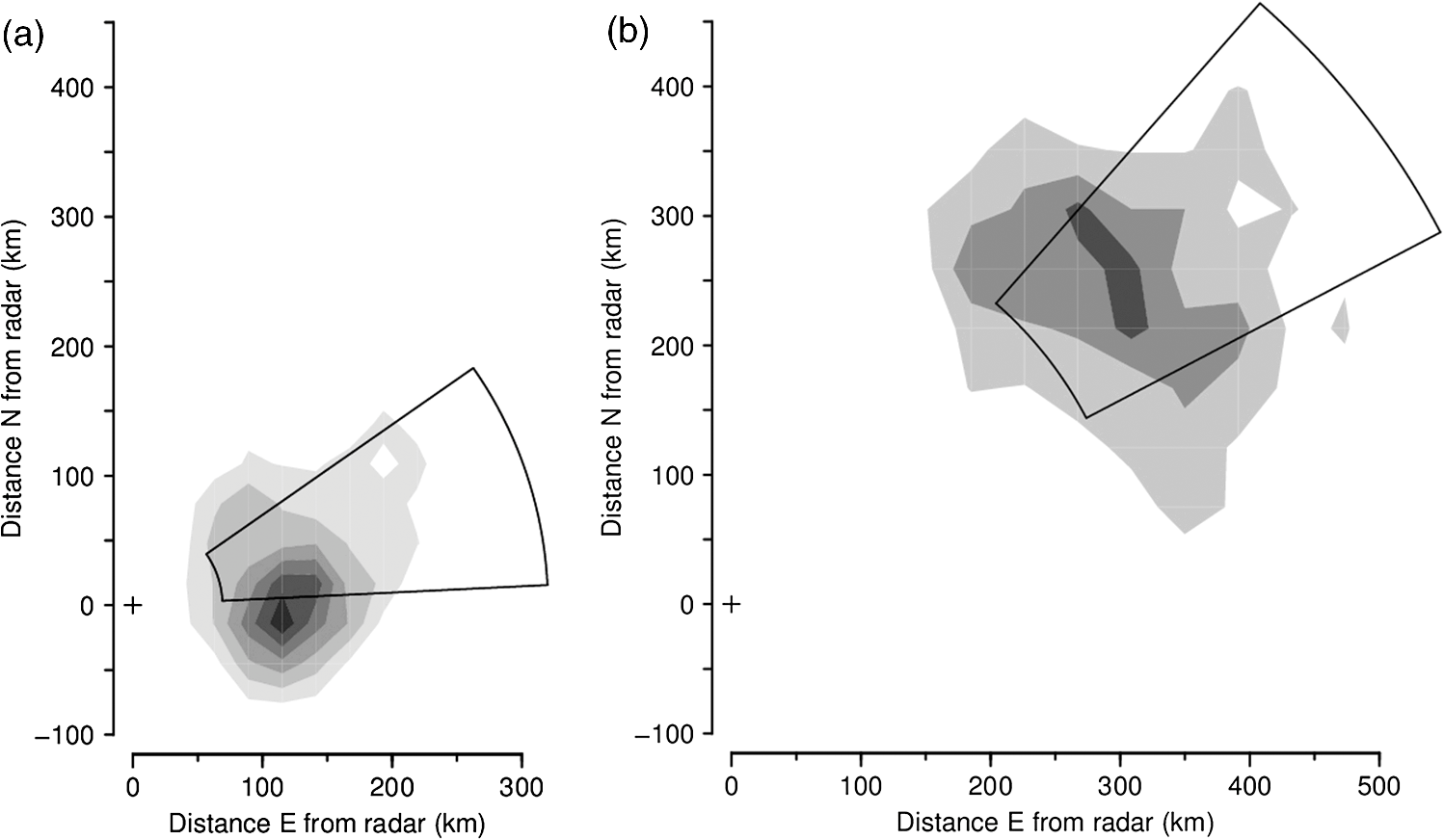

A more succinct indication of the source regions can be obtained by combining some of the statistical measures of each night’s migration that have already been calculated. In this approach, minimum distances are estimated from the 25-percentile speed for the target class and the start time of the phase (2 h for transmigration and 7 h for immigration) and maximum distances from the 75-percentile speed and either the finish time of the phase or its duration (as determined by a fall in the detection rate to $< 10 %$ of the average for the night, as in the analysis of Fig. 6(a)] if this is earlier. The range of directions is determined by the 25% and 75% quantiles of the direction distribution, and the intensity of migration by the number of targets detected during the phase. The source regions estimated in this way for the night of 17 to 18 March 2008 are superimposed on the contour plots of Fig. 7. There is generally reasonable agreement, although the poor range resolution arising from the 4- or 5-h long phase being treated as a single entity is apparent. A similar analysis can be made for destination regions, with populations detected during the emigration and transmigration phases being forward tracked to estimate their likely position around dawn. However, as the duration of the flights beyond the time of observation is unknown, the distances calculated constitute an upper limit rather than an estimate of position as in the source-region case.

Source regions calculated from the nominal durations of the phases and the 25- and 75-percentile statistics are shown for nights with high counts of C. terminifera-type targets in Fig. 8. Only regions for declared transmigration or immigration events are shown, and for clarity only the nine nights with $LI > 3.15$ (i.e., with at least 1413 fully analyzed targets exhibiting all C. terminifera characters) are included. The first of these was on 26 and 27 February, when the transmigration from the north-northeast was followed by an immigration from the north. The last was on 2 and 3 April when there was a transmigration from the north-northwest, the most intense recorded in this period, but no immigration event was declared. An analysis like those of Figs. 3 and 5 showed that the movement direction changed to eastward at around 01 h (and after $\sim 02 h$ was towards the northeast) and that target numbers fell sharply with the direction change. Five of the nine selected nights occurred during the period 15 to 24 March, with source regions to the southeast, east, northeast, and north of the radar. The movement of 7 and 8 March, from the south, was notably fast with speeds of 16 to $20 {ms}^{- 1}$ ; the movement of 11 and 12 March, from the east, was rather slow (7 to $10 {ms}^{- 1}$ ) during the immigration phase although speeds had been a more typical 9 to $12 {ms}^{- 1}$ earlier in the night. The immigration event on 17 and 18 March showed the greatest distance of movement in this sample, the estimated source region extending from 300 to 600 km; however, the more detailed analysis of this night presented in Fig. 7(b) indicates that few insects flew further than 400 km. This small, single-season study shows a predominance of movements with a westward component; this is consistent with previous analyses, drawing on data from earlier years, of C. terminifera-type targets at this site²⁴ [which is at the eastern edge of the region where the seasonal northward and southward movements⁴ predominantly occur]. The movements from the east can be attributed to the populations recorded by conventional methods at a distance of $\sim 300 km$ in that direction and fledging during this period (see above).

Fig. 8

Source areas estimated from statistical measures and nominal phase durations for declared transmigration (solid line) and immigration (dashed line) events identified from observations made with the Bourke IMR for the nine nights during the period of February to April 2008 for which the LI exceeded 3.15. Events were declared, and source regions identified, on the basis of observations of all large targets. The number of targets in each event is indicated by the thickness of the lines and ranged from 27 to 64 per minute of observation.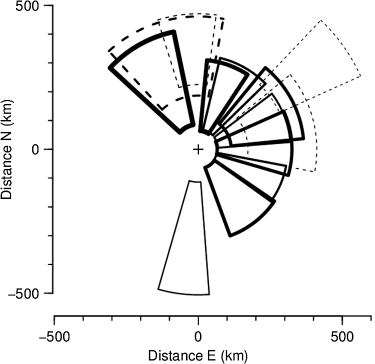

5. Discussion

The examples presented here illustrate both the potential value and the limitations of ground-based radar as a component of an information system for locust management. Foremost among the advantages of the units employed in the current work is that they operate automatically, require only occasional maintenance effort, and have modest running costs. These economies arise partly because they are installed permanently, so that the considerable redeployment effort associated with a mobile unit is avoided; the downside, of course, is that the radars are not always located in regions with active locust populations. A permanently installed unit provides a season-long time series of insect flight activity, and this will reveal upsurges and population movements more clearly than successive short periods of observations from a series of locations, however well placed these may be. Fixed units can play a sentinel role, detecting unforeseen movements and revealing previously unknown populations. The appropriate response to the challenge of the large area within which locust populations can develop therefore appears not to be use of mobile radars, but rather extension of the network of permanently installed units: another four to six radars have been suggested for C. terminifera monitoring in eastern Australia.¹³ These relatively simple radars are not so costly that this proposal is unrealistic, but it would constitute a significant capital item for a locust-control organization and a full-time specialist position would be needed to support the network and interpret the observations.

While IMRs provide useful information about the target type, this does not amount to a firm identification. Interpretation of the radar data therefore requires judgment based on knowledge of the migratory insect fauna of the region and the likely phenologies of the various species. The target characters (size, shape, wing-beat frequency) may be inferred from observations of similar species¹³ and then gradually confirmed through experience and “ground-truthing”, i.e., information from locust surveys and reports that corresponds with what the radar has detected. In an operational context, the radar outputs are best regarded as indicative. This is certainly the current practice of APLC, which always seeks confirmation of identity from other sources (landholder reports, light traps, or survey).

Some caution and a degree of judgment are also required when interpreting the indicated source and destination regions, as ground speeds and track directions at points along the trajectory will generally differ from those observed with the radar as the insects pass over. The most significant contributor to the insects’ velocities is the wind, and trajectories will curve, or exhibit sudden direction changes, if the wind field over the region is nonuniform or changing. The extent of variation of target speed and direction at the radar site (Fig. 3) can provide an indication of whether the flow is settled, and by inference whether it is uniform, but does not provide completely reliable information about the movement velocity elsewhere. For example, the change in direction from westward to south-westward evident in Fig. 3 was not necessarily experienced by any individual migrant: rather, those arriving early may well have remained in a westward-moving flow all night, and those arriving later may have been traveling south-westward since taking off.

The IMR observations alone do not allow true back-tracking,³⁹ which is best achieved using information about the wind field over the whole extent of the migrant’s trajectory. The wind data will derive from meteorological observations over a wide area and typically be provided in the form of outputs from numerical weather-forecasting analyses. If wind-field information is available, it can be drawn on to estimate source and destination regions;⁶ the IMR speeds and directions would then be relegated to a validation role and to provide an alert when the meteorological analysis is inaccurate. (The latter is most likely to occur when weather features like fronts or troughs are passing through, as the timing of these relative to dusk can be critical, or when small-scale disturbances like storm outflows and katabatic winds,¹³ that are confined to the lowest few hundred meters of the atmosphere, develop.) The IMR counts of target numbers remain, of course, the only source of information about migration intensities and their variation through the night, and hence about the appropriate durations for forward- and back-track calculations. Wind field information would also allow investigation of the effects on the trajectory of the locusts’ own airspeeds and their headings. However, this is more of interest to researchers than to operational forecasters for whom the stand-alone IMRs may be more practicable to operate and maintain than a system that requires data from two quite different sources to be merged.

The source regions estimated here are simply those for insects passing over the radar site. As the radar is sampling a broad-scale migration, the source population can be expected to extend laterally beyond the demarcated areas. Although no information is available for specific individual movements, some inferences can be drawn from the time variation of insect numbers along the migration direction, which the radar provides with a time resolution of $\sim 0.3 h$ . As can be seen in Fig. 5, periods of more intense migration typically persist for at least 2 h. At typical migration speeds of $\sim 10 m / s$ , this corresponds to a minimum spatial extent of source populations of $\sim 70 km$ : a scale comparable with that of the widths of the estimated source regions (Fig. 8). It would therefore seem unwarranted to broaden the area of any confirmatory searches (using ground or air patrols) much beyond the indicated source (or, more likely, destination) regions. The corollary of this is that populations $\sim 100 km$ or more to one side of the indicated source area are unmonitored by the radar. Information about these may become available in the following days if the direction of movement (i.e., of the wind) changes appropriately; alternatively, and more reliably, additional radars installed in a network with a spacing of 100 to 200 km should provide good day-by-day coverage. In the case of the present study, a predominantly westward movement direction allowed a fledging population to the east to be revealed but provided no indication of a second one to the west (see above).

The examples presented here demonstrate that continuous observation of migration at a single location provides quite rich information about the intensity and form of the movements there. However, the extent to which information can be drawn out is critically dependent on the size of the sample of targets. When the numbers are low, partitioning the sample both by time (1-h periods) and height (150-m intervals), as in the analyses of Figs. 3 and 5, leads to a high proportion of statistically insignificant results. While on a night of intense migration the number of detected targets is high ( $\sim 40,000$ ), many of these are not capable of being fully analyzed (because they pass too far to one side of the beam’s center or simply because the insects are too small). Of those echoes for which a full set of parameters is retrieved, many will prove to be of types that are of no interest to the ultimate user (e.g., a locust-control organization). At least with C. terminifera, further losses arise because a wing-beat frequency cannot be retrieved from many of the echoes. For these reasons, even on nights of heavy migration, the total sample for targets meeting all the criteria for C. terminifera is no more than $\sim 3000$ with the current IMR observing procedures. This is adequate for full partitioning, but of course, it is not only the very highest intensity movements that need to be studied; a sample of 300 events, one-tenth of the extreme value, would produce very sparse results for time and height variations and would hardly allow immigration, transmigration, and emigration events to be recognized. For these reasons, some analyses (e.g., Figs. 7 and 8 here) are carried out using all large targets, not just those meeting the C. terminifera criteria. It is to be expected, however, that there will be occasions when the target characters (Fig. 1) show that two different types of large target are moving together, so this is not satisfactory as a general procedure. Sample sizes could be approximately doubled by maximizing the time scheduled for observing during each hour, at the cost of a significantly larger data-storage requirement. Obviously, this would have some benefits for the study of lesser movements, but even without it the key migration events during each season can be recognized and their characters determined.

Radars of the IMR type observe insects flying directly overhead and are therefore suitable only for monitoring broad-front migrations. They are useful for C. terminifera because the major movements of this species occur at night, with the individuals flying independently for up to several hundred kilometers (while in its daytime swarming flights, this locust typically moves only a few tens of kilometers).⁴⁰ They are also suitable for other species with similar flight behavior provided that these are large enough to produce a strong echo and are sufficiently numerous. The Australian units commonly detect movements of moths, especially in early spring, and are used to study these species (some of which are of economic importance) as well as locusts. For species like the desert locust, Schistocerca gregaria, that form swarms and that move long distances in these concentrations, a more conventional scanning radar configuration capable of carrying out surveillance over a wide area would be required. A swarm passing even only a kilometer away from a vertical-beam radar would not be detected. Swarms of desert locusts have been observed with scanning radars built for meteorological observations,⁴¹ and insect concentrations have been detected out to ranges of $\sim 30 km$ with the lower-cost scanning entomological radars sometimes used for migration research,¹³ but so far radars have not been deployed for operational detection of locust swarms. IMRs may still be of value for monitoring movements of solitaria-phase desert locusts⁴² and for any other species in which movement in swarms is not the dominant form of migration.

At APLC, observations from the two IMRs have been available to forecasters during around 10 seasons, including some with significant locust populations and control campaigns. They have been found useful principally for the immediacy of the information they provide on population movements and because their coverage can substitute, to a degree, for ground surveys when heavy rain or flooding makes roads impassable and when survey staff are assigned elsewhere (e.g., to a control campaign). Perhaps their most significant contribution, however, has been as one of the sources of evidence that led to the recognition that northward flights of C. terminifera in late spring and early summer, previously dismissed as insignificant, are an important element of the species’ annual cycle.⁴ These “return migrations” are now understood to “seed” the subtropical (summer rainfall) rangelands of the far inland where population build-up can be rapid and lead to an outbreak.⁵ This insight has strengthened APLC’s capacity to undertake strategic control and thus accumulation of long-term statistics by the IMRs has proved as valuable as their direct operational/sentinel role.

Acknowledgments

This research has been supported through grants from the Australian Research Council. I. T. Harman made major contributions to the development of the IMRs and to the procedure used to analyze their signals. The radars were largely built by UNSW Canberra workshop staff and maintained in reliable operation by S. Hatty. Bourke and Bulloo Shire Councils have provided sites suitable for long-term installation and logistical support.

References

1.

E. D. DevesonP. W. Walker, “Not a one-way trip: historical distribution data for Australian plague locusts support frequent seasonal exchange migrations,” J. Orthopt. Res., 14 (1), 91 –105 (2005). http://dx.doi.org/10.1665/1082-6467(2005)14[91:NAOTHD]2.0.CO;2 JOREDR 0736-0266 Google Scholar

2.

K. J. Walden, “Insect migration in an arid continent. III. The Australian plague locust Chortoicetes terminifera and the native budworm Helicoverpa punctigera in Western Australia,” Insect Migration: Tracking Resources through Space and Time, 173 –190 Cambridge University Press, Cambridge (1995). Google Scholar

3.

G. LoveD. Riwoe, “Economic costs and benefits of locust control in eastern Australia,” (2005). Google Scholar

4.

E. D. Devesonet al., “Evidence from traditional and new technologies for northward migrations of Australian plague locusts (Chortoicetes terminifera) (Walker) (Orthoptera: Acrididae) to western Queensland,” Austral Ecol., 30 (8), 928 –943 (2005). http://dx.doi.org/10.1111/aec.2005.30.issue-8 1442-9985 Google Scholar

5.

D. E. Wright, “Analysis of the development of major plagues of the Australian plague locust Chortoicetes terminifera (Walker) using a simulation model,” Aust. J. Ecol., 12 (4), 423 –438 (1987). http://dx.doi.org/10.1111/aec.1987.12.issue-4 AJECDQ 1442-9993 Google Scholar

6.

D. M. HunterE. D. Deveson, “Forecasting and management of migratory pests in Australia,” Entomologia Sinica, 9 (4), 13 –25 (2002). Google Scholar

7.

D. M. Hunter, “Advances in the control of locusts (Orthoptera: Acrididae) in eastern Australia: from crop protection to preventive control,” Aust. J. Entomol., 43 (3), 293 –303 (2004). http://dx.doi.org/10.1111/aen.2004.43.issue-3 1326-6756 Google Scholar

8.

P. M. Symmons, “Control of the Australian plague locust, Chortoicetes terminifera (Walker),” Crop Protection, 3 (4), 479 –490 (1984). http://dx.doi.org/10.1016/0261-2194(84)90029-2 CRPTD6 0261-2194 Google Scholar

9.

V. A. DrakeR. A. Farrow, “The nocturnal migration of the Australian plague locust, Chortoicetes terminifera (Walker) (Orthoptera: Acrididae): quantitative radar observations of a series of northward flights,” Bull. Entomol. Res., 73 (4), 567 –585 (1983). http://dx.doi.org/10.1017/S0007485300009172 BEREA2 0007-4853 Google Scholar

10.

V. A. Drakeet al., “Characterizing insect migration systems in inland Australia with novel and traditional methodologies,” Insect Movement: Mechanisms and Consequences, 207 –233 CABI Publishing, Wallingford, UK (2001). Google Scholar

11.

V. A. Drake, “Automatically operating radars for monitoring insect pest migrations,” Entomologia Sinica, 9 (4), 27 –39 (2002). Google Scholar

12.

V. A. DrakeH. K. WangI. T. Harman, “Insect monitoring radar: remote and network operation,” Comput. Electron. Agric., 35 (2–3), 77 –94 (2002). http://dx.doi.org/10.1016/S0168-1699(02)00024-8 CEAGE6 0168-1699 Google Scholar

13.

V. A. DrakeD. R. Reynolds, Radar Entomology. Observing Insect Flight and Migration, CABI, Wallingford, UK (2012). Google Scholar

14.

A. D. SmithJ. R. RileyR. D. Gregory, “A method for routine monitoring of the aerial migration of insects by using a vertical-looking radar,” Philos. Trans. R. Soc. London B, 340 (1294), 393 –404 (1993). http://dx.doi.org/10.1098/rstb.1993.0081 PTRBAE 0962-8436 Google Scholar

15.

I. T. HarmanV. A. Drake, “Insect monitoring radar: analytical time-domain algorithm for retrieving trajectory and target parameters,” Comput. Electron. Agric., 43 (1), 23 –41 (2004). http://dx.doi.org/10.1016/j.compag.2003.08.005 CEAGE6 0168-1699 Google Scholar

16.

H. K. WangV. A. Drake, “Insect monitoring radar: retrieval of wingbeat information from conical-scan observation data,” Comput. Electron. Agric., 43 (3), 209 –222 (2004). http://dx.doi.org/10.1016/j.compag.2004.01.003 CEAGE6 0168-1699 Google Scholar

17.

V. A. Drake, “Signal processing for ZLC-configuration insect-monitoring radars: yields and sample biases,” in Radar 2013. 2013 Int. Conf. Radar, 9-12 September 2013, Adelaide, South Australia, (2013). Google Scholar

18.

J. W. Chapmanet al., “Development of vertical-looking radar technology for monitoring insect migration,” Comput. Electron. Agric., 35 (2–3), 95 –110 (2002). http://dx.doi.org/10.1016/S0168-1699(02)00013-3 CEAGE6 0168-1699 Google Scholar

19.

G. W. Schaefer, “Radar observations of insect flight,” Insect Flight (Symposia of the Royal Entomological Society no. 7), 157 –197 Blackwell Scientific, Oxford (1976). Google Scholar

20.

S. E. HobbsA. C. Aldhous, “Insect ventral radar cross-section polarisation dependence measurements for radar entomology,” IEE Proc. Radar Sonar Navigation, 153 (6), 502 –508 (2006). http://dx.doi.org/10.1049/ip-rsn:20060019 1350-2395 Google Scholar

21.

T. J. DeanV. A. Drake, “Monitoring insect migration with radar: the ventral-aspect polarization pattern and its potential for target identification,” Int. J. Remote Sens., 26 (18), 3957 –3974 (2005). http://dx.doi.org/10.1080/01431160500165955 IJSEDK 0143-1161 Google Scholar

22.

J. R. Riley, “Radar cross section of insects,” Proc. IEEE, 73 (2), 228 –232 (1985). http://dx.doi.org/10.1109/PROC.1985.13135 IEEPAD 0018-9219 Google Scholar

23.

V. A. DrakeI. T. HarmanH. K. Wang, “Insect monitoring radar: stationary-beam operating mode,” Comput. Electron. Agric., 35 (2–3), 111 –137 (2002). http://dx.doi.org/10.1016/S0168-1699(02)00014-5 CEAGE6 0168-1699 Google Scholar

24.

H. K. Wang, “Evaluation of insect monitoring radar technology for monitoring locust migrations in inland Eastern Australia,” School of Physical, Environmental & Mathematical Sciences, University of New South Wales, Canberra, 2008). Google Scholar

25.

T. J. Dean, “Development and evaluation of automated radar systems for monitoring and characterising echoes from insect targets,” School of Physical, Environmental & Mathematical Sciences, University of New South Wales, Canberra, Australia, 2007). Google Scholar

26.

G. McDonaldK. P. BrycesonR. A. Farrow, “The development of the 1983 outbreak of the common armyworm, Mythimna convecta, in eastern Australia,” J. Appl. Ecol., 27 (3), 1001 –1019 (1990). http://dx.doi.org/10.2307/2404392 JAPEAI 1365-2664 Google Scholar

27.

P. C. GreggA. P. Del SocorroR. A. Rochester, “Field test of a model of migration of moths (Lepidoptera: Noctuidae) in inland Australia,” Aust. J. Entomol., 40 (3), 249 –256 (2001). http://dx.doi.org/10.1046/j.1440-6055.2001.00228.x 1326-6756 Google Scholar

28.

V. A. DrakeR. A. Farrow, “A radar and aerial-trapping study of an early spring migration of moths (Lepidoptera) in inland New South Wales,” Aust. J. Ecol., 10 (3), 223 –235 (1985). http://dx.doi.org/10.1111/aec.1985.10.issue-3 AJECDQ 1442-9993 Google Scholar

29.

D. P. Clark, “Flights after sunset by the Australian Plague locust, Chortoicetes terminifera (Walk.), and their significance in dispersal and migration,” Aust. J. Zool., 19 (2), 159 –176 (1971). http://dx.doi.org/10.1071/ZO9710159 AJZOAS 0004-959X Google Scholar

30.

D. M. Hunter, “Mass take-off after sunset in the Australian plague locust,” Australian Plague Locust Commission Annual Report 1979-1980 Research Supplement, 68 –72 Australian Plague Locust Commission, Canberra (1981). Google Scholar

31.

C. G. Johnson, Migration and Dispersal of Insects by Flight, Methuen, London (1969). Google Scholar

32.

G. A. BartholomewB. Heinrich, “A field study of flight temperatures in moths in relation to body weight and wing loading,” J. Exp. Biol., 58 (1), 123 –135 (1973). JEBIAM 0022-0949 Google Scholar

33.

G. McDonaldR. A. Farrow, “Migration and dispersal of the Rutherglen bug, Nysius vinitor Bergroth (Hemiptera: Lygaeidae), in eastern Australia,” Bull. Entomol. Res., 78 (3), 493 –509 (1988). http://dx.doi.org/10.1017/S0007485300013249 BEREA2 0007-4853 Google Scholar

34.

Locust Bulletin, Australian Government Department of Agriculture, Fisheries and Forestry, Canberra (2013). Google Scholar

35.

V. A. Drake, “The vertical distribution of macro-insects migrating in the nocturnal boundary layer: a radar study,” Boundary-Layer Meteorol., 28 (3–4), 353 –374 (1984). http://dx.doi.org/10.1007/BF00121314 BLMEBK 0006-8314 Google Scholar

36.

V. A. DrakeR. A. Farrow, “The influence of atmospheric structure and motions on insect migration,” Annu. Rev. Entomol., 33 183 –210 (1988). http://dx.doi.org/10.1146/annurev.en.33.010188.001151 ARENAA 0066-4170 Google Scholar

37.

N. I. Fisher, Statistical Analysis of Circular Data, Cambridge University Press, Cambridge (1993). Google Scholar

38.

“Compute Sunrise, Sunset & Twilight Times,” (2013). http://www.ga.gov.au/geodesy/astro/sunrise.jsp Google Scholar

39.

J. W. Chapmanet al., “Flight orientation behaviors promote optimal migration trajectories in high-flying insects,” Science, 327 (5966), 682 –685 (2010). http://dx.doi.org/10.1126/science.1182990 SCIEAS 0036-8075 Google Scholar

40.

R. A. Farrow, “Offshore migration and the collapse of outbreaks of the Australian plague locust (Chortoicetes terminifera Walk.) in South-east Australia,” Aust. J. Zool., 23 (4), 569 –595 (1975). http://dx.doi.org/10.1071/ZO9750569 AJZOAS 0004-959X Google Scholar

41.

B. V. Ramana-Murtyet al., “Observations on flying locusts by radar,” J. Sci. Ind. Res., 23 289 –296 (1964). JSIRAC 0022-4456 Google Scholar

42.

J. R. RileyD. R. Reynolds, “Vertical-looking radar as a means to improve forecasting and control of desert locusts,” in New Strategies in Locust Control (Proc. Int. Conf. New Strategies in Locust Control, Bamako, Mali, 3–8 April 1995, 47 –54 (1997). Google Scholar

Biography

V. Alistair Drake received BA and DPhil degrees in physics at Oxford University, UK, before transferring his research to the fields of radar entomology and insect migration. In 1978, he moved to Australia, working initially with the Commonwealth Scientific and Industrial Research Organisation’s Division of Entomology and later as an academic with The University of New South Wales at its Canberra campus. His research has focused especially on the development of radar techniques for insect observation, the relation of insect migration to atmospheric phenomena, migration as an adaptation to environments that vary both spatially and with time, and the application of entomological radars to operational pest forecasting. He is a coauthor of a recently published monograph on radar entomology. Now retired, he continues his research through associations with both UNSW Canberra and the Institute of Applied Ecology at the University of Canberra.

Haikou Wang received a BSc in agricultural entomology and an MSc in insect ecology from Nanjing Agricultural University, China, before moving to The University of New South Wales at its campus in Canberra, Australia, where he completed a PhD on the use of Insect Monitoring Radars for observing migrations of Australian plague locusts. After postdoctoral research on windborne dispersal of money spiders at Cambridge University, UK, he took up a position at the Australian Plague Locust Commission in Canberra, Australia, where his responsibilities include managing the GIS and interpreting the remote-sensing (satellite imagery and entomological radar) and meteorological (winds, temperatures, rainfall) data streams.

CC BY: © The Authors. Published by SPIE under a Creative Commons Attribution 4.0 Unported License. Distribution or reproduction of this work in whole or in part requires full attribution of the original publication, including its DOI.

Citation Download Citation

V. Alistair Drake and Haikou Wang "Recognition and characterization of migratory movements of Australian plague locusts, Chortoicetes terminifera, with an insect monitoring radar," Journal of Applied Remote Sensing 7(1), 075095 (5 September 2013). https://doi.org/10.1117/1.JRS.7.075095

Published: 5 September 2013

Access the abstract

JOURNAL ARTICLE
18 PAGES

DOWNLOAD PAPER SAVE TO MY LIBRARY

GET CITATION

CITATIONS

Cited by 29 scholarly publications.

Explore citations on Lens.org

KEYWORDS

Radar

Target detection

Lithium

Statistical analysis

Motion analysis

Knowledge management

Polarization

1.

Introduction

2.

Insect Monitoring Radars

3.

Locust Identification