Detecting annual and seasonal changes in a sagebrush ecosystem with remote sensing-derived continuous fields

Collin G. Homer; Debra K. Meyer; Cameron L. Aldridge; Spencer J. Schell

doi:10.1117/1.JRS.7.073508

9 September 2013 Detecting annual and seasonal changes in a sagebrush ecosystem with remote sensing-derived continuous fields

Collin G. Homer, Debra K. Meyer, Cameron L. Aldridge, Spencer J. Schell

Author Affiliations +

Journal of Applied Remote Sensing, Vol. 7, Issue 1, 073508 (September 2013). https://doi.org/10.1117/1.JRS.7.073508

Abstract

Climate change may represent the greatest future risk to the sagebrush ecosystem. Improved ways to quantify and monitor gradual change resulting from climate influences in this ecosystem are vital to its future management. For this research, the change over time of five continuous field cover components including bare ground, herbaceous, litter, sagebrush, and shrub were measured on the ground and by satellite across six seasons and four years. Ground-measured litter and herbaceous cover exhibited the highest variation annually and herbaceous cover the highest variation seasonally. Correlation of ground measurements to corresponding remote-sensing predictions indicated that annual predictions tracked ground measurements more closely than seasonal ones, and QuickBird predictions tracked ground measurements more closely than Landsat predictions. When annual linear slope values from ground plots and sensor predictions were correlated by component, the direction of ground-measured change was tracked better with QuickBird components than with Landsat components. Component predictions were correlated to annual and seasonal DAYMET precipitation. QuickBird components on average had the best response to precipitation patterns, followed by Landsat components. Overall, these results demonstrate the ability of sagebrush ecosystem components as predicted by regression trees to incrementally measure changing components of a sagebrush ecosystem.

1. Introduction

Sagebrush (Artemisia spp.) ecosystems constitute the single largest North American semiarid shrub ecosystem¹ and provide vital ecological, hydrological, biological, agricultural, and recreational ecosystem services.²^,³ However, disturbances such as livestock grazing, exotic species invasion, conversion to agriculture, urban expansion, energy development, and other development have historically altered and reduced these ecosystems,²^,⁴^–⁶ with $\sim 50 %$ loss in total spatial extent.³^,⁷^,⁸ Constant perturbations and changes to these systems are disrupting vital biological services, such as providing habitats for numerous sagebrush-obligate species, including the sage-grouse (Centrocercus spp.). This has severely affected sage-grouse populations across their ranges,³^,⁹ leaving populations threatened with extirpation in some habitats where they historically persisted.³^,¹⁰

While ecosystem-wide disturbances are having diverse impacts to sagebrush habitats today, climate change may ultimately represent the greatest future risk to this ecosystem.¹¹^–¹⁴ Both warming temperatures and changing precipitation patterns (such as increased winter precipitation falling as rain) will likely favor species other than sagebrush¹⁵ and increase sagebrush disturbance risk from fire, insects, diseases, and invasive species.¹¹^,¹⁶ Despite the vast area covered by this ecosystem and the numerous disturbance forces operating on the landscape, effective large-area monitoring and prediction tools have not been implemented, and widely accepted metrics to quantify and communicate disturbance magnitudes are not well developed.¹⁷^–²⁰ Disturbance monitoring capable of measuring, quantifying, and reporting change in metrics understood by land managers is critical to future successful management of this ecosystem.³^,¹⁰^,¹⁸^,²¹^,²²

Optical remote sensing is still the most likely data source and tool for large-area monitoring of disturbance within the sagebrush ecosystem, supporting a framework that can offer relatively efficient and accurate analysis of change across a range of spatial and temporal scales.²¹^,²³^,²⁴ Sagebrush ecosystems represent a challenging remote-sensing environment because these semiarid shrublands have sparse and similar vegetal cover with high proportions of bare ground and a variety of soil reflectance properties.²⁵^,²⁶ Despite these challenges, an optical remote-sensing signal capable of characterization exists for semiarid shrublands, and monitoring is feasible.²⁶^–³² Studies within the sagebrush ecosystem have demonstrated the ability for remote sensing to characterize more abrupt types of disturbance from fire³³^,³⁴ and human development³⁵^,³⁶ and gradual types of disturbance such as grazing³⁷ and climate change.²³

A comprehensive understanding of the relationship between remote-sensing change and gradual changes in sagebrush ecosystem components is still lacking; only a few studies have begun to explore that relationship.²⁴^,³⁶^,³⁸^–⁴⁰ Further, even beyond the sagebrush ecosystem to semiarid systems in general, remote-sensing change studies have historically targeted the development of indices such as the normalized difference vegetation index (NDVI) or other similar approaches to understand change.⁴¹^–⁴³ These indices can be difficult to interpret and translate to on-the-ground understanding.⁴⁴^–⁴⁶

Metrics that characterize changes that managers readily use in the field for real-time decisions, such as fractional vegetation predictions,²¹ would more likely ensure application of such products for daily management decisions and applications. Recent research has sought to reconcile this need, with approaches centered on using a single year of training data to parameterize a base characterization layer, which is then projected through several time periods using change vector analysis to identify what change is occurring. This approach assumes change areas identified in the change vector process can be labeled using values from the base characterization layer.³⁹^,⁴⁰ However, no research has tested this assumption by gathering repeated ground measurements over many time steps (seasons or years) to fully evaluate the ability of the change vector approach to detect fine-scale change within sagebrush ecosystems.

Technological advances have also resulted in the development of higher-spatial-resolution sensors offering new potential for monitoring in sagebrush ecosystems at resolutions finer than Landsat.¹⁹^,²¹^,⁴⁷^–⁴⁹ New spectral bands at finer spatial resolution can increase our ability to detect smaller changes and improve monitoring applications. Increased sensor resolution may allow for changes to be detected at more local scales, enhancing interpretation and understanding. Also, because ground-measurement approaches are often prohibitively expensive, high-resolution sensors offer the potential to extrapolate ground measurement across larger landscape models and also provide an operational surrogate for ground plot remeasurement. However, studies that explore the capabilities of higher-resolution sensors to complement and support component predictions derived at moderate spatial scales for change monitoring have not been completed.

Downscaling of climate information such as precipitation also continues to evolve to better support more localized analysis. The release of new data with longer temporal records and at finer spatial scales provides new opportunities for defining the relationship between climate change and sagebrush ecosystem change. Specifically, the new release of DAYMET daily gridded surface climate data,⁵⁰ providing daily precipitation data at a 1-km spatial resolution, provides a new opportunity to explore potential finer-scale links of climate change to any observed ecosystem change.

We attempt to address these research gaps by capitalizing on advancements in high-resolution remote-sensing data availability, remote-sensing component prediction and change detection, and new availability of higher-spatial-resolution precipitation. Our goal was to explore whether component change and precipitation impacts can be detected across multiple scales of remote sensing in a sagebrush ecosystem. Ongoing ground and satellite monitoring of several focus areas in Wyoming provide the opportunity to explore change patterns from a variety of drivers. For this evaluation, we focus on one particular monitoring site, labeled “1.” Site 1 has had no observed potential change drivers during field visits or in any satellite images other than climate influences during the timeframe of this study, offering a good opportunity to examine ecosystem change driven only by variation in climatic conditions. We tracked component change in this sagebrush ecosystem across 4 years and six seasons (during the first 2 years) using multiyear satellite imagery and ground-based vegetation sampling. The spatial distribution and temporal change for fractional cover components of bare ground, herbaceous, litter, shrub, and sagebrush were quantified between 2008 and 2011. Our specific study objectives were to (1) determine the relationship between changing spatial and temporal extents of fractional component change as measured from three scales, including ground measurement, QuickBird (QB) 2.4-m satellite acquisitions, and Landsat 5 (LS) 30-m satellite acquisitions; (2) quantify, compare, and contrast observed changes of remote-sensing sagebrush ecosystem components across years and seasons with ground measurements; (3) test if remote-sensing components trained on a single base year (2008), and subsequently extended through time using change vector analysis (2009 to 2011), are sensitive enough to capture subtle ground-measured change over time; and (4) use DAYMET precipitation data to evaluate if precipitation changes correlate with annual and seasonal component change identified from ground measurement, QB predictions, and LS predictions.

2. Data and Methods

2.1.

Overview

Our approach examined 2 years of seasonal sagebrush ecosystem change nested within 4 years of annual sagebrush ecosystem change using data collected from ground measurements and remote-sensing data from QB and LS. We measured proportional amounts of each of five sagebrush ecosystem fractional cover components (hereafter simply called components) including cover of bare ground, herbaceous, litter, sagebrush (all species), and shrub (all shrubs combined) as continuous fields in 1% intervals using both ground plots and satellite predictions. Using 2008 ground measurements, we produced QB and LS satellite data component predictions for the study area. The percent cover of each component was then both annually and seasonally updated only in areas that had spectrally changed from the 2008 base year or season. These updates were completed with regression trees (RT) using unchanged 2008 base areas as training sources. We collected field data in other years and seasons for evaluation of these predictions. Correlation analysis was then conducted to explore relationships between various ground, satellite, and precipitation measurements. We explain each methodological step by section below.

2.2.

Study Area

The study was conducted in southwestern Wyoming, United States. One $64 - {km}^{2}$ area (site 1) was selected as a focus area for intensive ground measurement coupled with QB and LS measurements (Fig. 1). This site represented one of 30 sites used for initial 2006 Wyoming sagebrush characterization.²¹ Site 1 is located $\sim 22 km$ southeast of Farson, Wyoming. It contains a range of topography with elevations from 2026 to 2327 m, and slopes up to 31 deg. It has predominantly sandy soils and contains part of the Farson sand dunes in the northeast corner. Vegetation is dominated by sagebrush shrubland, especially in the upland areas, with salt desert shrub species dominating in the lowland and sandy areas. Herbaceous areas range from typical grasses and forbs interspersed among shrubs to subirrigated meadows where a high subsurface water table in the sand dune areas creates higher-than-normal biomass productivity for these selected areas. This site is public land administered by the Bureau of Land Management and is typically grazed by cattle most of the summer. During our study, we observed no substantial differences in the amount or duration of grazing from year to year.

Fig. 1

Location and spatial extent of the study area site 1 used for monitoring sagebrush component change from 2008 to 2011 in southwestern Wyoming.

2.3.

Baseline Data Collection

2.3.1.

Plot selection and measurement

We segmented the QB imagery into spectrally similar polygon patches to identify sites for potential ground sampling. We also classified the image into 30 unsupervised clusters. Segmented polygons were then intersected with the 30 clusters to identify the majority cluster class in each polygon, and 66 polygons representing the full range of spectral variability across the QB image were then selected.²¹ Ground measurements were conducted using ocular measurements at seven $1 - m^{2}$ quadrats along each of two 30-m transects within each polygon plot.²¹^,²⁷ To ensure remeasurement was spatially over the same quadrat areas, we permanently staked the beginning and ending of each transect. Cover was estimated from an overhead perspective (satellite), with the total cover of all vegetation and soil components summing to 100%. The shrub component represented all woody shrub species; the sagebrush component is a subset of the shrub component and represented only sagebrush shrub species (Artemisia spp.); the herbaceous component represented all grasses (live and residual standing) and forbs; litter is the combined cover of dead standing woody vegetation and detached plant and animal organic matter; and the bare ground component represented any exposed soil or rocks. All individual quadrat cover estimates were made in 5% increments. Ground measurements were conducted annually on the same approximate dates, with QB image acquisition attempted as near these dates as possible. Plot measurements for 2008 to 2011 were conducted by the same two individuals over the same plots every year, except in 2011 when the alternate observer sampled all plots.

2.3.2.

Image collection and preprocessing

QB images covering the study area were targeted seasonally (spring, summer, and fall) for 2008 and 2009, and annually during each of the summers of 2008 through 2011. Four-band multispectral images (visible blue, green, red, and near-infrared) were collected at 2.4-m resolution with a desired target of $< 20 \deg$ off-nadir view angle. Imagery was processed by Digital Globe to UTM using a $2 \times 2$ bilinear resampling kernel. We used the ERDAS 10 AutoSync tool to accomplish QB orthorectification using 1-m National Agricultural Imagery Program imagery as the base. The AutoSync tool uses an automatic point matching algorithm to generate hundreds of tie points between the reference image and the subject image to complete the geometric correction. This functionality is sensor specific and enhanced with the use of a digital elevation model (DEM). Subsequent years of QB imagery were registered to the orthorectified 2008 image base to ensure spatial consistency using the same process as described above. QB images were converted to at-sensor reflectance using the following equation:

ρ_{λ} = \frac{L_{λ} \times d^{2} \times π}{{Esun}_{λ} \times \cos (θ_{s})},

where

ρ_{λ} = planetary

top-of-the-atmosphere reflectance (unitless),

π = mathematical

constant equal to

\sim 3.14159

(unitless),

L_{λ} = spectral

radiance at the sensor’s aperture [

W / (m^{2} \cdot sr \cdot μm)

],

d = Earth-sun

distance (astronomical units),

{Esun}_{λ} = mean

exoatmospheric solar irradiance [

W / (m^{2} \cdot sr \cdot μm)

], and

θ_{s} = solar

zenith angle (deg).

This is similar to the approach used for converting the LS imagery to at-sensor reflectance.⁵¹^,⁵² Results were then converted to 8-bit files using a scaling factor of 400 to remain consistent with the way the LS was processed.

Multiseason and multiyear LS imagery from 2008 to 2011 was acquired for path 37 row 31 and processed using the automated level 1 product feneration system. Through this process, the scenes were converted to at-sensor reflectance, projected to Albers equal area, and terrain corrected.⁴⁰^,⁵²^–⁵⁴ The positional accuracy of all LS and QB images was carefully controlled to ensure direct comparisons of multiple dates and image platforms were spatially accurate.

2.3.3.

Component predictions

The 2008 base spatial distributions of five components of sagebrush habitat including cover of bare ground, herbaceous, litter, shrub, and sagebrush were estimated at 1% intervals for both QB and LS using RT models. For QB, 120 ground transects, with four additional mini plots centered over very high component value areas, were used for RT training. Vegetation characteristics were sampled at seven $1 - m^{2}$ quadrats along 30-m transects in sample polygons. The mean value for each of the variables of interest was calculated across all seven 1-m quadrats within a transect. These values were assigned to all pixels occurring within the sampling area for each transect. The five component predictions within the QB image were developed independently from multispectral QB and ancillary data using the RT algorithm Cubist¹^,⁵⁵ following a protocol developed in an earlier study.²¹ For LS, QB predictions from three sites (including site 1) across the LS thematic mapper (TM) scene were combined to build training data for the LS modeling. These additional sites provided variation in land cover types resulting in comprehensive training across the entire TM scene and replicated a typical full TM scene component modeling scenario.²¹ We purposely developed the LS prediction with the full TM scene perspective to ensure that the predictions at site 1 represent a typical landscape level application. We refined the training by dividing the data for each of the five component predictions into roughly three equal bins based on the mean and root mean square error (RMSE). The middle bin was thinned more relative to the other bins to ensure that higher and lower component values carried appropriate weighting in the model development and reduced overall bias. LS predictions were modeled using one leaf-on image from each year for annual predictions and one seasonal image from each season of each year for seasonal predictions, coupled with DEM ancillary data.

2.3.4.

Image normalization and change identification

The process of normalizing many image dates to ensure consistent comparison is important for initiating trend analysis. Once images are normalized, potential change areas need to be identified and the magnitude and type of change labeled. We accomplished this process by following several major processing steps. For QB, all cloud and cloud shadow areas in the scenes were masked and excluded to ensure these areas did not incorrectly influence the normalization outcome. Next, NDVI was calculated for each image, and a difference layer was calculated, to compare NDVI magnitude differences between the reference scene (from 2008) and the subject scene. Experimental trials of different NDVI thresholds revealed that a threshold of $\pm 5$ NDVI values was appropriate for excluding outlier pixels from influencing the normalization process. This process of outlier pixel exclusion ensured normalization was developed from only the most invariant pixels. Finally, a linear regression algorithm was developed from the invariant pixels and used to relate each pixel of the subject image to the reference image (2008 image) band by band.⁴⁰ For LS, a similar approach was followed. First, all cloud, cloud shadow, and snow and ice areas were excluded from analysis. Then, a normalization procedure using a linear regression algorithm to relate each pixel of the subject image to the reference image (2008 leaf-on) band by band was conducted.⁴⁰

Once image normalization was completed, images across years and seasons were compared for identification of change areas using a change vector process. For QB, change pixels were determined using a standard deviation (SD) from the mean value. Pixels outside 1 SD were considered to be potential change areas. LS change pixels were determined using thresholds specific to general land cover classes spatially identified from the 2006 National Land Cover Database.⁴⁰ Change areas identified with the threshold approach tended to be too conservative to capture all change relative to field measurements, and an additional independent approach was necessary to further capture potential change areas with more subtle change. This additional approach used NDVI differencing between the master scene (2008) and the subject year or season to confirm change pixels. Research trials showed that pixels outside of $\pm 5$ NDVI values for QB and outside of $\pm 3$ values for LS needed to be retained as change pixels (the greater sensitivity of QB to image noise artifacts necessitated a higher threshold than LS to maintain comparability across sensors). The final potential change mask was created combining (union) both the change vector process and the NDVI differencing results. All cloud and cloud shadow areas were treated as no change areas and removed from the change mask image.

Labeling annual and seasonal subsequent change areas with the new component values was accomplished for both QB and LS by using an RT modeling approach and input data layers similar to that used to predict the 2008 baseline distributions. Training data were gathered from the 2008 unchanged baseline component values after first excluding potential change pixels by using the change masks described above. A random sample of 10,000 points for QB and 25,000 points for LS were selected from candidate pixels for each component. Predictions quantifying the spatial distribution and per-pixel proportion of five components as a continuous variable were then calculated using regression models for all change pixels in each QB and LS image. Baseline predictions for spectrally unchanged pixels were not modeled and were left as original predictions from the base year. Using the change mask created from the change vector process, each of the change pixel prediction values was then applied over the base prediction. The no-change pixels retained the prediction value from the base prediction, and only the change pixel areas were updated for each new imagery date.⁴⁰

2.4.

Data Analysis and Evaluation

2.4.1.

Data summation and analysis protocols: plot-level polygon data

Both QB and LS predictions were evaluated by comparison to corresponding ground plot measurements within plot polygons and analyzed by component and data source. Component values measured at ground plots were compiled into a single mean transect value (seven individual frames on a 30-m transect) for comparison to QB, and by plot (two transects, 14 individual frames) for comparison to LS. Similarly, for QB and LS predictions, all pixel values within each ground plot polygon or transect boundary were averaged to represent one component value for each transect/plot (referred to simply as plot hereafter). For consistency, the exact same plots were analyzed across all years and seasons. If clouds or other image issues precluded a plot from inclusion from one year or season, it was eliminated from analysis from all dates. This ensured fair comparisons between sensors and components. For each annual and seasonal plot, the SD of the individual frame measurements was calculated. For each annual plot, a slope value from a linear regression was also calculated. In order to facilitate direct comparison among components and data sources, the coefficient of variation (COV) ( $m ean / SD \times 100$ ) was also calculated for each plot.

To determine whether significant change had occurred on ground-measured annual and seasonal plots, a one-way analysis of variance (ANOVA) was performed. This calculation uses the SD from the individual transect frame measurements for each plot to determine whether there are any significant differences between the means of plot measurements across time. All ANOVA significance levels are reported at $alpha = 0.1$ . To determine if a significant direction of change occurred on annual plots, the linear slope was calculated and significance tested at the 0.1 level.

Several combinations of Pearson’s correlation were used to compare ground plot measurements to QB and LS predictions. First, in order to test the overall similarity of the component predictions to ground measurements, a correlation analysis comparing plot-level mean component values for each of the data sources was completed. Second, correlation was used to test the strength of the relationship between ground-measured significant ANOVA plots and significant slope plots to component predictions. Finally, correlation of slope values from both ground measurements and component predictions was used to test the ability of components to track the direction of change over time.

2.4.2.

Data summation and analysis protocols—by total proportional area

To test component prediction relationships beyond plot-level polygons, ground measurements, QB and LS predictions were also compiled to assess the total area of change of components across the full study area. For ground-measured polygons within the site 1 study area, the total area covered by all polygons was calculated; subsequently, the proportion of that total area covered by each component by year and season was also calculated. For QB and LS, the full study extent of site 1 predictions were used to calculate the areal proportion of each component of each cell into a total area summary value (e.g., a 50% bare ground prediction in a 30-m LS cell means 50% of the area of that cell is counted as bare ground, or $450 m^{2}$ ). The mean proportional amounts of total area by year and season were calculated for each data source. We calculated the mean epoch-to-epoch percent change by dividing the percent change of epoch (season or year) by the total number of epochs, and also calculated the mean relative error between component predictions and ground measurement. Pearson’s correlation analysis was used to compare proportional component measurements among data sources.

2.4.3.

Comparison to precipitation, by source and component

DAYMET daily gridded surface climate data providing daily precipitation data at a 1-km spatial resolution was downloaded for site 1 for 2008 to 2011.⁵⁰ Daily data were then combined into mean seasonal precipitation amounts by 1-month and 2-month intervals for seasonal analysis, and by calendar year and water year (September to October) for annual analysis. Mean monthly and annual DAYMET precipitation values for all cells in site 1 were then pooled into a single mean value representing the entire site 1 study area. Corresponding mean monthly and annual total area percent component values from ground measurements and QB and LS predictions for site 1 were then correlated with precipitation data using Pearson’s correlation.

3. Results

3.1.

Overview

We measured five sagebrush ecosystem fractional cover components including bare ground, herbaceous, litter, sagebrush, and shrub on the ground and from satellites over six seasons and four years. Comparison analysis of component change patterns among data sources was conducted at both the single-plot level and proportionally across the entire study area. Study area proportional seasonal and annual changes were also correlated to annual and seasonal precipitation measurements. Specific results are listed by section below.

3.2.

Plot-Level Ground and Satellite Measurements

A total of 66 ground plots (132 transects) were sampled during the summers of 2008 through 2011 across site 1. Only plot results from 2008 were used to develop RT predictions for all five components across one 2.4-m QB $64 - {km}^{2}$ image extent (site 1) and corresponding LS extent; all other years and seasons were developed using change vector analysis (Fig. 2). The RMSE average for the 2008 base estimate for all five components over site 1 was 4.68 for QB and 6.83 for LS.²¹ Image collection dates deviated an average of 16 days from ground collection for QB and nine days from ground collection for LS (Table 1). After removing plots affected by clouds on either QB or LS imagery, 52 plots (104 transects) remained for analyses.

Fig. 2

Site 1 QuickBird (QB) (2.4 m) on the left and Landsat 5 (LS) (30 m) 2008 base component predictions on the right. Masked cloud areas in the LS predictions are shown in gray. Note the total range of each component prediction.

Table 1

Ground-measurement dates, with corresponding Landsat and QuickBird image collection dates.

Source	Spring 2008	Summer 2008	Fall 2008	Spring 2009	Summer 2009	Fall 2009	Summer 2010	Summer 2011	$\bar{x}$ (days) from field collection	SE
Ground	June 17	July 22	Sept 22	June 13	July 22	Sept 22	July 14	July 16
QB	-----	Aug 11	Oct 17	June 3	July 14	Sept 14	July 12	Aug 21	16	4.5
LS	June 20	July 22	Sept 24	June 23	Aug 10	Sept 27	Aug 13	July 14	9	3.9

Of the five components, litter exhibited the highest COV for annual ground-measured change at 18.4, with herbaceous second at 18.1, then shrub at 17.2, sagebrush at 9.9, and bare ground the lowest at 8.3 (Table 2, Fig. 3). Litter had the largest number of plots qualifying as significantly changed from the ANOVA analysis at 15, with herbaceous second at 13, bare ground third at 7, and shrub and sagebrush with 1 each (Table 2). Only seven annual plots overall showed significant plot change and significant slope change, two each in bare ground and litter, and one in each of the remaining three components.

Table 2

Mean ground-measured annual change (% of 100) across 52 plots, by component.

Components	Plots ( $N$ )	2008 (mean)	2009 (mean)	2010 (mean)	2011 (mean)	SD (mean)	Coefficient of variation (mean)	Linear slope	$N$ with sig. ANOVA (.10)	$N$ with sig. slope (.10)
Bare ground	52	57	54	56	55	2.88	8.3	1.36	7	2
Herbaceous	52	16	16	15	14	2.42	18.1	1.31	13	1
Litter	52	16	17	16	16	1.94	18.4	0.79	15	2
Shrub	52	11	12	12	13	1.45	17.2	0.76	1	1
Sagebrush	52	6	7	7	8	0.99	9.9	0.53	1	1

Fig. 3

Visual example of bare ground component change in the northeastern part of site 1 from 2008 through 2011 in southwestern Wyoming. QB bands 4, 3, and 2 are displayed as RGB on the left, and the corresponding bare ground component predictions are on the right.

For seasonal change, herbaceous exhibited the highest COV for ground-measured change at 23.8, with litter second at 21.4, then sagebrush at 19.4, shrub at 18.9, and bare ground the lowest at 8.7 (Table 3). Litter and herbaceous had the largest number of plots with significant ANOVA-measured change at 23 each, with bare ground next at 11, then shrub with 2, and sagebrush with 1 (Table 3).

Table 3

Mean ground-measured seasonal change (% of 100) across 52 plots, by component.

Component	Plot $N$	June 2008 (mean)	July 2008 (mean)	Sept 2008 (mean)	June 2009 (mean)	July 2009 (mean)	Sept 2009 (mean)	SD (mean)	Coefficient of variation (mean)	$N$ with sig. ANOVA (.10)
Bare ground	52	59	57	57	56	54	56	3.42	8.7	11
Herbaceous	52	15	16	14	15	16	12	3.04	23.8	23
Litter	52	15	16	17	16	17	19	2.80	21.4	23
Shrub	52	11	11	11	12	12	12	1.67	18.9	2
Sagebrush	52	7	6	6	7	7	7	1.02	19.4	1

3.3.

Plot-Level Data Correlation Relationships

Each set of values from both annual and seasonal individual ground plots and transects were correlated with the corresponding satellite component measurements to test the ability of the component predictions to replicate ground measurements. Overall, annual predictions were more highly correlated than seasonal predictions, and QB had higher correlation values than LS (Table 4). QB displayed a mean correlation value across all components of 0.85 for annual and 0.82 for seasonal. LS had a mean correlation value of 0.77 across all components for annual and 0.73 for seasonal. For components, bare ground had the highest mean correlation across sensors at 0.91, with shrub exhibiting the lowest correlation at 0.69 (Table 4).

Table 4

Remote-sensing prediction correlations to annual and seasonal ground measurements over plot areas, by component.

Component	$N$		Annual		Seasonal
Component	QB (transects)	LS (plots)	QB ( $R$ )	LS ( $R$ )	QB ( $R$ )	LS ( $R$ )	Mean
Bare ground	104	52	.94	.92	.90	.88	.91
Herbaceous	104	52	.81	.73	.81	.71	.77
Litter	104	52	.93	.87	.87	.80	.87
Shrub	104	52	.77	.63	.75	.59	.69
Sagebrush	104	52	.78	.71	.77	.69	.74
Mean			.85	.77	.82	.73

Note: All correlations were significant at the 0.01 level.

The linear slope value was calculated across annual measurements for each plot, QB and LS prediction. These slope values were then correlated to test the ability of component predictions to replicate the trend of ground-measured slope change. QB had relatively high correlation values for individual components, and most correlations were significant (Table 5). In contrast, LS had low correlation values for individual components, with significant correlation values only in the bare ground component. When slope values from all plots and transects were pooled across all components ( $N = 520$ ), QB had a correlation of 0.37 and LS a correlation of 0.10. When a subset of slope values from only significant ground-measured ANOVA plots were pooled (Table 2) ( $N = 40$ ), QB had a correlation of 0.74 and LS remained at 0.10. However, correlation of slope values from ground-measured plots with a subset of both significant ANOVA and slope results ( $N = 14$ ) yielded a correlation of 0.77 for QB and a correlation of 0.64 for LS (Table 5).

Table 5

Annual component correlations of individual linear slope value calculated for plot measurements, correlated with the linear slope value calculated for corresponding LS and QB predictions.

	QuickBird		Landsat
Component stratification (ANOVA and slope significance from field measurements)	$N$ (Transect)	$R$	$N$ (Plot)	$R$
Bare ground—all plots	104	.28a	52	.23a
Bare ground—only plots ANOVA significant at 0.1	9	.78a	7	.73a
Bare ground—only plots slope significant at 0.1	3	.92	2	+
Herbaceous—all plots	104	.70a	52	$- .06$
Herbaceous—only plots ANOVA significant at 0.1	15	.78a	13	.10
Herbaceous—only plots slope significant at 0.1	8	.86a	1	+
Litter—all plots	104	.61a	52	.05
Litter—only plots ANOVA significant at 0.1	13	.78a	15	.23
Litter—only plots slope significant at 0.1	1	+	2	+
Shrub—all plots	104	$- .46$ a	52	.13
Shrub—only plots ANOVA significant at 0.1	3	$- .99$ a	1	+
Shrub—only plots slope significant at 0.1	2	+	1	+
Sagebrush—all plots	104	$- .55$ a	52	$- .07$
Sagebrush—only plots ANOVA significant at 0.1	0	+	1	+
Sagebrush—only plots slope significant at 0.1	0	+	1	+

All components, all plots combined	520	.37a	260	.10
All components, only significant ANOVA plots combined	40	.74a	37	.10
All components, only significant slope plots combined	14	.77a	7	.64

Note: Correlation results reveal the ability of the sensor component predictions to replicate the direction of slope change as measured on the ground.Note: +Inadequate sample size.

^aCorrelation significant at 0.1.

3.4.

Total Area Comparison

The total proportional area covered by each component from each source (ground and satellite) was calculated for each season and year across all of site 1, with the proportion of change between seasons and years also calculated. For annual predictions, bare ground exhibited the highest mean annual change at 1.3%, shrub the next highest at 0.8%, then herbaceous at 0.6%, litter at 0.5%, and sagebrush the lowest at 0.3% (Table 6). Shrub had the highest mean annual relative error, and litter had the lowest. When compiled by data source, ground measurement showed the highest overall mean change across all components at 1.02%, with LS second at 0.56%, and QB the lowest at 0.52%. Ground mean annual change values showed the most variation between components, with QB showing the least. Overall, QB had higher relative errors than LS (Table 6).

Table 6

Comparison of the percent proportions of total area covered by each component for every year.

Component	2008	2009	2010	2011	Mean annual change (%)	Mean annual relative error (%)
Bare ground (%)
Field	59.5	57.1	59.1	57.8	1.9
QuickBird	59.7	59.1	59.9	60.6	0.7	2.5
LS	60.3	61.4	60.8	58.8	1.2	3.4
Mean					1.3
Herbaceous (%)
Field	15.7	15.9	13.5	13.3	0.9
QB	12.9	13.3	12.8	12.7	0.3	10.9
LS	13.2	12.5	12.9	13.7	0.6	9.6
Mean					0.6
Litter (%)
Field	15.4	16.1	14.8	15.5	0.9
QB	15.3	15.7	15.6	15.2	0.3	0.1
LS	15.4	15.2	15.4	16.2	0.4	0.7
Mean					0.5
Shrub (%)
Field	10.2	11.9	12	12.7	0.8
QB	9.6	10.4	9.1	10.2	1.1	15.6
LS	10.1	9.8	10.0	10.8	0.4	12.4
Mean					0.8
Sagebrush (%)
Field	5.8	7.1	7.3	7.6	0.6
QB	5.4	6.1	6.1	6.0	0.2	14.7
LS	6.2	6.2	6.3	6.8	0.2	7.4
Mean					0.3

Note: For ground plots, the total area is calculated from pooling all plot polygons; for QB and LS, the total area is calculated from full study area predictions.

For seasonal measurements, the mean total proportional seasonal change across six seasons for ground and LS and five seasons for QB was calculated. Bare ground exhibited the highest mean seasonal change at 2.0%, herbaceous next at 1.2%, litter at 0.8%, shrub at 0.7%, and sagebrush the lowest at 0.5% (Table 7). Herbaceous had the highest mean annual relative error, and bare ground had the lowest. When compiled by data source, in contrast to annual measurements, LS showed the highest overall mean seasonal change across all components at 1.90%, with ground second at 0.7%, and QB the lowest at 0.52%. The seasonal change values showed the most variation between components from LS, with QB showing the least. Overall, LS had higher relative errors than QB (Table 7).

Table 7

Comparison of the percent proportions of total area covered by each component for every season.

Component	June 2008	July 2008	Sept 2008	June 2009	July 2009	Sept 2009	Mean seasonal change (%)	Mean annual relative error (%)
Bare ground
Field	61.4	59.9	60.1	58.5	57.8	58.8	0.9
QB	—^a	59.9	60.7	59.8	59.5	62.4	1.2	2.4
LS	57.0	60.6	60.7	55.7	61.8	65.6	3.8	1.4
Mean							2.0
Herbaceous
Field	13.4	14.0	13.3	14.0	14.3	12.0	1.0
QB	—^a	12.8	11.9	12.6	13.0	11.7	0.8	8.4
LS	13.7	12.8	12.3	14.4	12.2	10.4	1.7	6.7
Mean							1.2
Litter
Field	13.8	15.5	15.6	15.3	16.2	17.8	0.7
QB	—^a	15.6	15.7	15.8	15.7	14.9	0.3	2.9
LS	16.8	15.4	15.8	17.8	15.3	14.2	1.5	2.0
Mean							0.8
Shrub
Field	10.0	09.6	10.1	11.0	11.1	10.8	0.5
QB	—^a	10.4	10.3	10.4	10.4	10.0	0.2	1.6
LS	11.9	10.1	10.4	12.5	09.9	09.1	1.5	2.5
Mean							0.7
Sagebrush
Field	06.5	05.6	05.7	06.9	06.8	06.6	0.4
QB	—^a	06.1	06.3	06.2	06.1	06.1	0.1	1.6
LS	07.8	06.3	06.7	08.2	06.3	06.4	1.0	10.2
Mean							0.5

Note: For ground plots, the total area is calculated from pooling all plot polygons; for QB and LS, the total area is calculated from full study area predictions.

^aNo data collected.

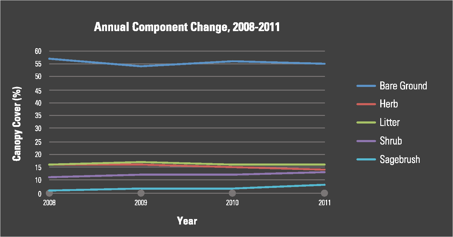
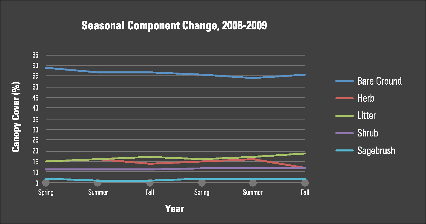
3.5.

Total Area Correlation to Precipitation Data

DAYMET annual precipitation at site 1 varied from a low of 219 mm in 2009 to a high of 297 mm in 2011 (Fig. 4), with seasonal scenarios varying from a low of 2 mm in August/September 2008 to a high of 67 mm in June 2008 (Fig. 5). Correlation of mean monthly and annual DAYMET precipitation values to the corresponding mean monthly and annual total area component calculations is presented in Table 8. Of the 60 scenarios tested, only nine were significant at the 0.1 level. When correlations were averaged across components, herbaceous had the highest mean correlation across all seasonal and annual scenarios at 0.67, and shrub the lowest at 0.47. When correlations were averaged by data source, the highest mean correlation was LS annual water year at 0.88, and the lowest was LS seasonal bimonthly correlation at 0.29 (Table 8). The highest significant individual correlation scenario was ground plot herbaceous against calendar year precipitation at $- 0.99$ .

Fig. 4

Annual precipitation measurements for site 1, compiled by calendar year and water year, in millimeters.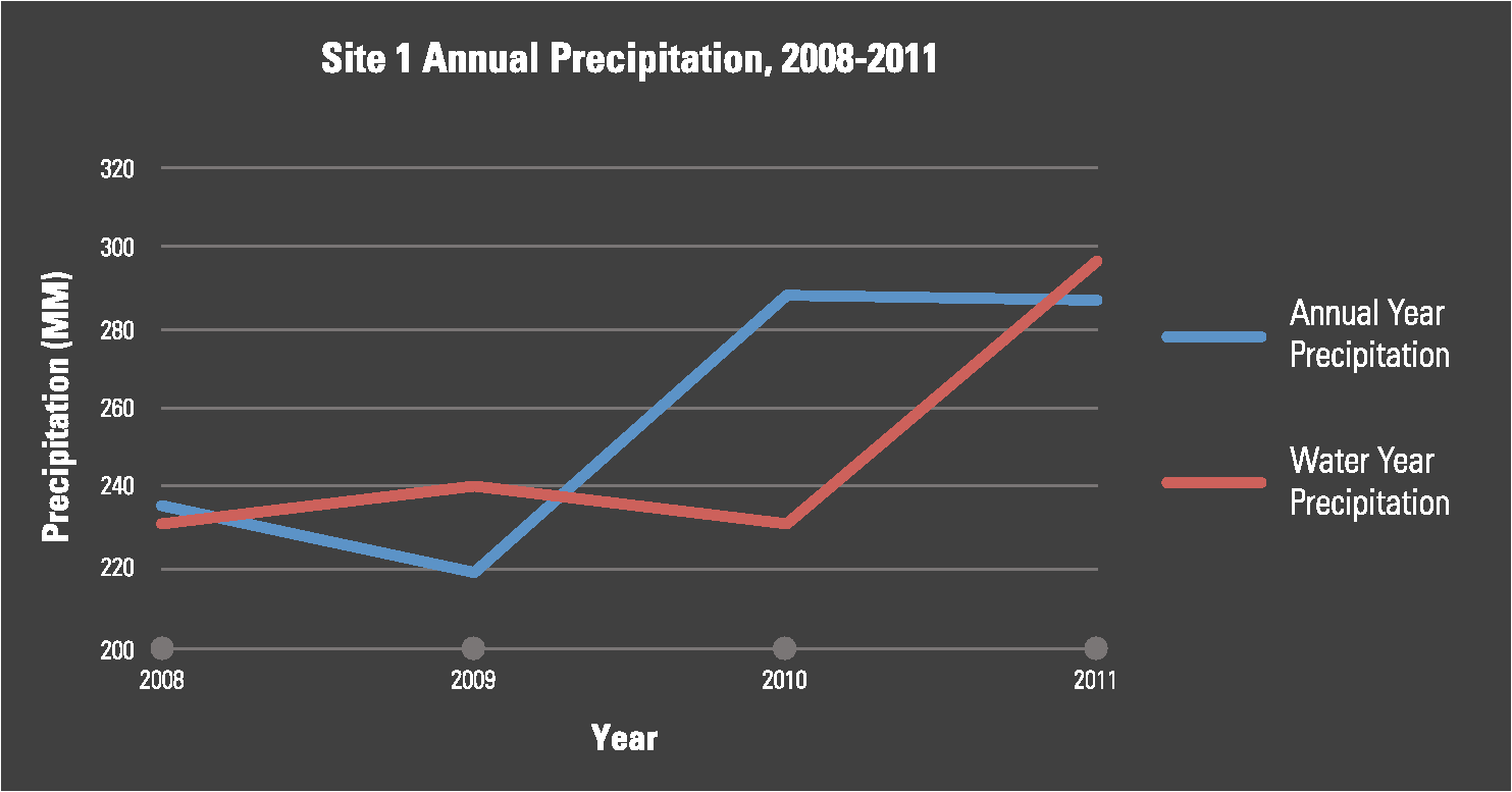

Fig. 5

Seasonal precipitation measurements for site 1 compiled both monthly and bimonthly, in millimeters.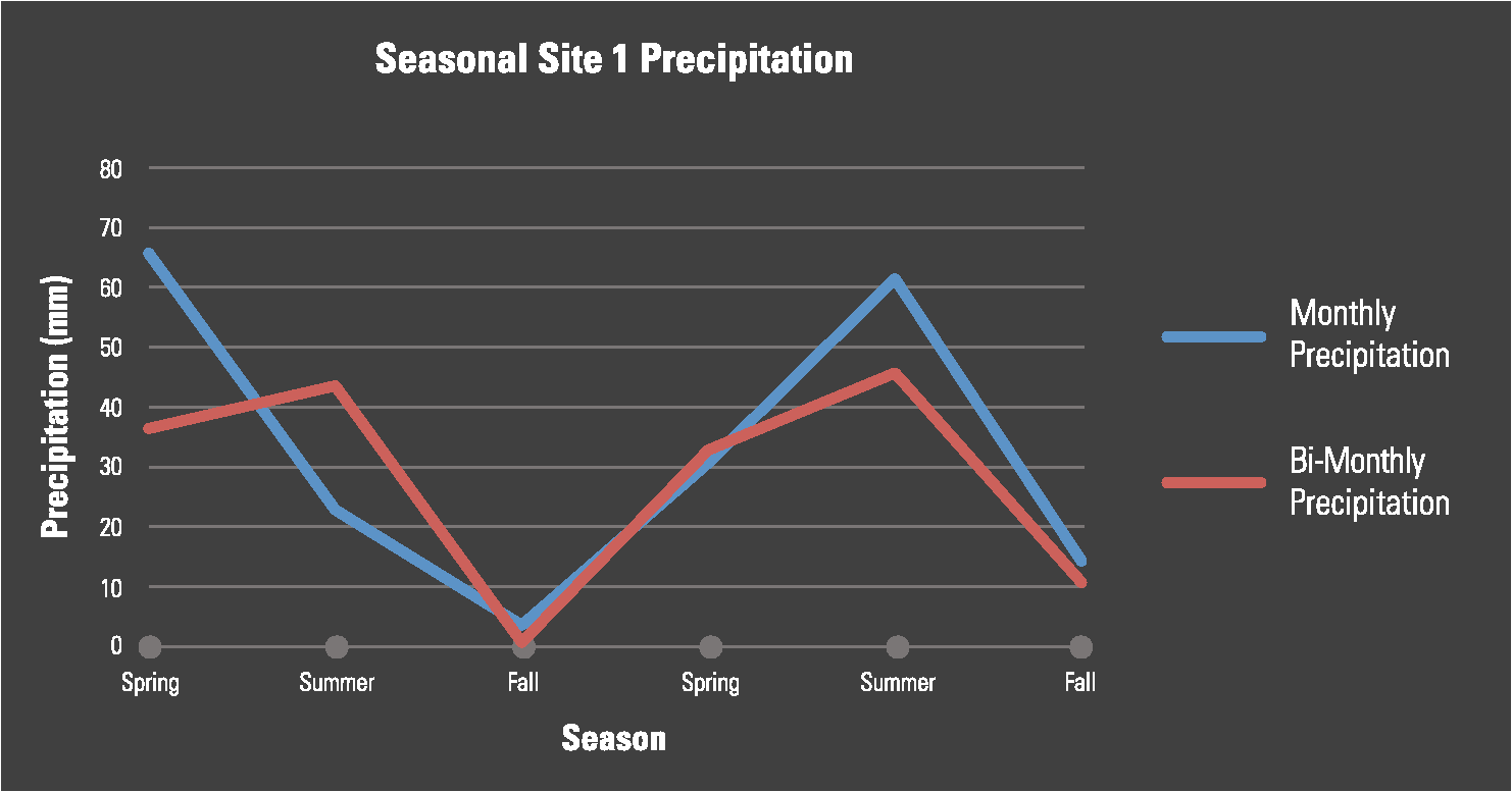

Table 8

Correlation (R) of annual and seasonal precipitation measurements over site 1 to corresponding annual and seasonal component change from ground plots and sensor predictions.

	Ground plots, site 1				QB, site 1				LS, site 1
Component	Seasonal		Annual		Seasonal		Annual		Seasonal		Annual
Component	Month of ground sample	Bi month of ground sample	Calendar year	Water year (Oct to Sep)	Month of ground sample	Bi month of ground sample	Calendar year	Water year (Oct to Sep)	Month of ground sample	Bi month of ground sample	Calendar year	Water year (Oct to Sep)	Mean
Bare ground	.04	$- .14$	.26	$- .46$	$- .62$	$- .75$ a	.87	.77	$- .38$	$- .38$	$- .60$	$- .86$	.51
Herbaceous	.47	.74a	$- .99$ a	$- .56$	.82a	.95a	$- .90$ a	$- .47$	.37	.47	.62	.72	.67
Litter	$- .49$	$- .39$	$- .76$	.17	.35	.42	$- .53$	$- .70$	.28	.26	.65	.95a	.50
Shrub	.21	.01	.55	.66	.49	.60	.46	.52	.34	.26	.66	.93a	.47
Sagebrush	.54	.27	.55	.60	−.60	−.65	.38	.33	.28	.09	.72	.95a	.50
Mean	.35	.31	.62	.49	.57	.67	.63	.56	.33	.29	.65	.88

^aCorrelation significant at 0.1.

4. Discussion

Our results demonstrate reasonable ability of sagebrush ecosystem components as predicted by regression trees to incrementally measure changing components of a sagebrush ecosystem. Specifically, we demonstrate the ability of regression tree component predictions to track ground-measured change over time using ground data from one year and change vector analysis for subsequent years. We demonstrate the ability of high-spatial-resolution satellite imagery to serve as a potential surrogate for repeated ground measurement. Finally, we demonstrate the ability of component predictions to potentially monitor vegetation change related to precipitation variation over time. Specific discussion topics are covered below.

4.1.

Ground-Measured Component Change

Ground measurements reveal a subtle changing landscape both seasonally and annually (Tables 2 and 3). This is to be expected given that we could observe no other major change agent operating in this area, other than climate.²³^,⁴⁰ However, it is encouraging that we were able to observe and detect this subtle change from both a ground and remote-sensing perspective. We went to great lengths to ensure ground measurements were consistent by using staked plots, revisiting plots at the same time of year and season, and having the same observer repeat measurements. The only exception was from 2011, when 35 plots were measured by the alternate observer; however, a quality check of these data revealed the measurement pattern to be consistent with previous measurements both observers had completed.

Component change varied by season and year, with seasonal measurements in every component consistently showing a higher COV than annual measurements (Fig. 6). This follows an expected ecosystem pattern, with seasonal plant response potentially more dynamic than annual response.⁵⁶^,⁵⁷ For individual components, litter and herbaceous exhibited the highest COV from annual measurements, and herbaceous the highest for seasonal measurements. These results are logical due to the ephemeral nature of these components with changing precipitation.⁵⁶ The shrub and sagebrush components exhibited relatively moderate COVs in both seasonal and annual measurements, with sagebrush having a substantially lower annual COV than shrub (Fig. 6). Sagebrush species contain some ephemeral leaves, which are dropped later in the growing season,⁵⁸^,⁵⁹ and we suspect this change is detected on the seasonal plots from spring measurement, but not on summer-measured annual plots. Alternatively, the shrub component contains many additional shrub species besides sagebrush that exhibit sustained growth through the entire season, resulting in similar change patterns for both annual and seasonal measurements. Because of the relatively high SD exhibited by bare ground, we did not anticipate that it would have the lowest COV of any component in both seasonal and annual measurements (Tables 2 and 3). However, high proportions of bare ground on many of our plots resulted in a large dynamic range for this measurement, which was factored out by the COV, suggesting bare ground in site 1 had relatively low variation both seasonally and annually compared to other components.

Fig. 6

Mean individual ground-measured coefficient of variation values, compiled annually and seasonally by component.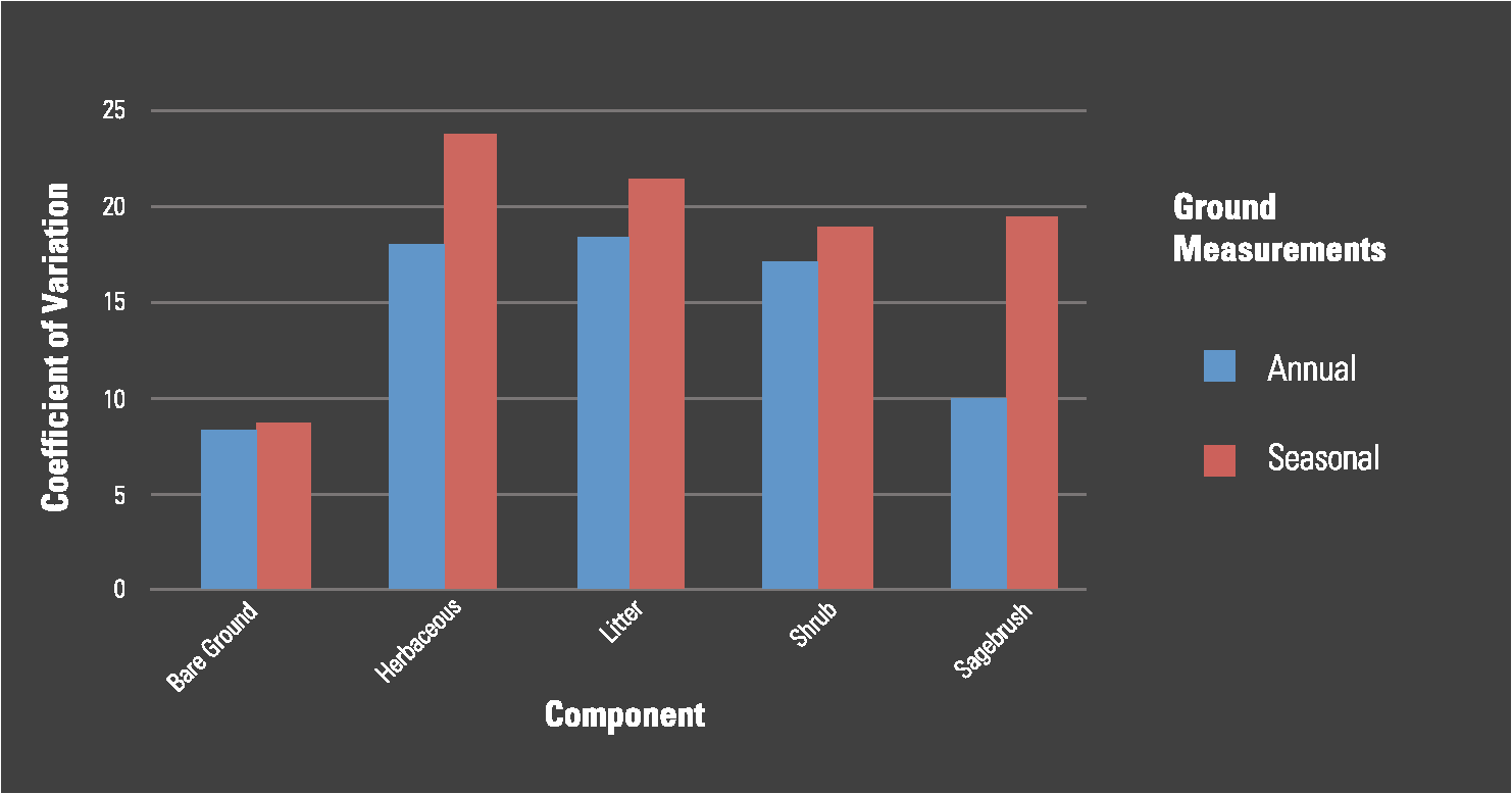

Overall, total annual changes were represented by a gradual increase in shrub and sagebrush canopy with corresponding decreases in bare ground, herbaceous, and litter across the four years (Fig. 7). Given that water year precipitation increased from 231 to 297 mm over this time, this type of component response makes sense for shrub, sagebrush, and bare ground. The slow growth of the sagebrush is to be expected; others have reported that multiple precipitation years may be required to influence overall growth.¹ We expected to see larger annual fluctuations of herbaceous cover, but given the annual growth pattern of many of the herbaceous plants,⁵⁶^,⁶⁰ it would appear that herbaceous cover in this case is mostly responding to the seasonal precipitation pattern rather than the annual. Total seasonal component change patterns show seasonal fluctuations, especially for the more ephemeral components of bare ground, herbaceous, and litter (Fig. 8). These seasonal patterns are also reflected in the annual patterns from the overall 2-year annual trends of decreasing bare ground and herbaceous, increasing litter, slightly increasing shrub, and stable sagebrush. The timing of the moisture of the second year (2009) being less abundant in the spring, and more abundant (Fig. 8) later in the summer, appears to also have influenced the more ephemeral components, with bare ground and herbaceous showing a noticeable fluctuation, and litter a noticeable increase.

Fig. 7

Total annual ground-measured percent change compiled by component, 2008 to 2011.

Fig. 8

Total seasonal ground-measured percent change compiled by component, 2008 to 2009.

4.2.

Satellite Acquisitions

Detecting subtle change with remote sensing requires rigorous processing protocols to overcome inconsistencies in satellite measurements from atmospheric conditions, sun-sensor geometry, geolocation error, variable ground pixel size, sensor noise, vegetation phenology, and surface moisture conditions.⁴⁵ We paid careful attention to processing protocols developed in this study as well as previous research²¹ to minimize potential noise differences. The greatest challenge was to ensure that timing of satellite collects were appropriate for ground-measured phenology conditions. As reported in Table 1, our high-resolution QB satellite collects were less phenologically accurate than LS because the variance from the timing of ground measurements was seven days greater. In this case, we feel the effects were minimal. But because our study area is semiarid with more minimal cloud cover than less arid places, gaining an appropriate phenological series of high-resolution imagery for potential monitoring in other places remains a challenge. Additionally, the need to collect appropriately timed imagery should not outweigh the need for collects with useable view angles. Our experience shows that acquiring high-resolution satellite collects with view angles of $< 20 \deg$ is the most desirable; greater angles make comparison across years or seasons more difficult because of distorted ground geometry. In our case, three QB images had view angles $> 20 \deg$ , which required extra processing to maintain consistency. This extra processing is a challenge and does affect product quality, but we recognize that the use of high-view angle imagery cannot always be avoided.

4.3.

Component Change Magnitude and Direction

With such subtle change amounts and a small sample size of years and seasons, gaining additional understanding of real change versus simple measurement variance is important. We approached this in two ways. First, we examined ground plot deviation using a one-way ANOVA that capitalized on examining the variance of the individual frame measurements for each plot. For annual plots, the mean variation (based on COV) for all pooled plots was 14.8, and the mean COV variation for significant ANOVA pooled plots was 36.4. For seasonal plots, the mean COV variation for all pooled plots was 18.4 and the mean COV for significant ANOVA pooled plots was 35.1. These results confirm that a higher variance threshold was required to achieve significant change and suggest that annual and seasonal average plot COVs of 35 or higher, on average, indicate that change on the plot is substantial enough to be real.

Second, we pooled ground plots by three categories (all plots, significant ANOVA plots, and significant ANOVA and slope value plots) with the corresponding sensor-based predictions to understand if our ability to capture change with imagery increased as the significance of change on the ground increased. We anticipated that the sensor-based component predictions would be more successful in capturing ground-measured change as the reliability and magnitude of change increases. Analysis reveals that as difference trends increase, there is a better correlation with imagery linear slope values (Fig. 9), suggesting that as more real change is realized on the ground, sensor component predictions perform increasingly better. QB especially performs well, suggesting a good ability to be a future surrogate for ground measurement, either supplementing or replacing ground plots under some circumstances. LS correlations only improved after pooling for slope significance, suggesting that ground component change needs to happen at both substantial spatial and temporal scales to be reliably detected by LS components.

Fig. 9

Three annual mean correlation comparison scenarios of individual ground-measured slope values correlated to the corresponding remote-sensing prediction slope values by data source. Scenarios include pooling of all ground-measured plots, a subset containing only those with significant analysis of variance (ANOVA) change, and a further subset containing only those with both significant ANOVA change and a significant slope change direction.

4.4.

Performance of Satellite Component Predictions

A key objective of this study was to test the utility of continuous field component predictions as a method capable of monitoring subtle change on a sagebrush ecosystem. Especially, this method depends on predictions created from a single base year (2008) or season and then identifies component change on subsequent periods using change vector analysis and RT labeling. When compared to corresponding ground measurements by correlation, sensor component predictions performed reasonably well, with mean $R$ values of 0.85 and 0.82 for QB, and 0.77 and 0.73 for LS, all significant at the 0.01 level (Table 4), successfully demonstrating this objective. We assume QB predictions outperformed LS largely due to the more compatible spatial scale in relationship to the ground plots and spatial ecology and pattern of vegetation in this ecosystem. QB predictions were trained and compared to ground data at the transect level (two transects in every plot) rather than plot level for the training and comparison of LS. The finer spatial scale of QB allowed better tracking of local heterogeneity that was more homogenized at the LS scale. In the future, some additional QB component performance improvement may be realized by training and monitoring at a finer spatial scale than demonstrated by our transect level; however, we speculate that at some level, complications of controlling spatial geometry, erratic plot variance, and spurious sensor variance could overwhelm any benefit.⁶¹^,⁶²

When sensor predictions over the entire study area (rather than only at plot level) were compiled as total proportions by component, the correlation of QB and LS proportional area estimates to corresponding ground proportional areas was very high ( $> 0.99$ ) for both annual and seasonal predictions, showing general compatibility among sources. Additionally, annual and seasonal component change relationships were very similar to plot-level polygon measurements, suggesting that sensor predictions over the entire study area remained reliable. For annual predictions, ground-measured proportions exhibited the highest amount of change, with LS second and QB the lowest, with QB also displaying the highest relative error (Table 6). We assume most change variance is scale related—likely a combination of variance from the ground-measurement method and the different ratio of total landscape area covered by ground polygons compared to QB or LS wall-to-wall predictions. Lower change numbers for sensor predictions over ground measurements could also indicate our change method was either too conservative, creating more omission than commission errors, or some ground change was not resolvable by the sensors. For seasonal predictions, LS showed the highest overall mean seasonal change, with ground measurement second and QB the lowest, although LS had higher relative error than QB (Table 7). LS seasonal change values also showed the most variation between components. This amount of change from LS was unexpected, as we anticipated QB to have higher change rates than LS, especially given the consideration that all LS classification and analysis was performed at the much broader landscape level. Our assumption that LS data in general were better calibrated and consistent, and warranted a lower NDVI change threshold than QB (3% versus 5%) for change vector component production, appears to be unlikely. This lower threshold likely contributed to the higher LS change values and relative error by allowing more commission error over actual unchanged areas than QB.

4.5.

Precipitation Correlation Results

We recognize that rigorous climate change analysis with remote-sensing predictions should ideally be done over spatial and temporal scales larger than our study area. However, this research offered the opportunity to compare annual and seasonal component series measured on the ground and by satellite to newly available DAYMET downscaled precipitation data, providing potential insight into the relationship between component change and precipitation change. Correlations of component change to precipitation change overall were better than expected. When individual component correlations to precipitation were averaged across all components by data source, QB had the highest mean correlations overall at 0.61, with LS having the next highest at 0.54, and ground the lowest at 0.44. The higher mean correlations from the sensor components over the ground measurements are likely due to the ability of their wall-to-wall prediction scale to provide better correlation to the 1-km cell precipitation data than the small footprint of ground plots.

When individual component correlations to precipitation were averaged across all components by season, the annual component mean correlation of 0.64 was much higher than the seasonal component mean correlation of 0.42, suggesting annual component predictions as a whole better reflected precipitation pattern than seasonal predictions. Closer examination of mean correlations pooled by individual annual components reveals mean values ranging from 0.71 for herbaceous to 0.64 for bare ground, 0.63 for shrub and litter, and 0.59 for sagebrush. The seasonal component mean values ranged from 0.64 for herbaceous to 0.41 for sagebrush, 0.39 for bare ground, 0.37 for litter, and 0.32 for shrub. This suggests that annual components of herbaceous, shrub, and sagebrush, and the seasonal component of herbaceous, have the greatest capacity to reflect precipitation patterns. However, component categories still need more in-depth precipitation analysis. For example, when individual component correlations to precipitation are pooled into two categories of ephemeral (bare ground, herbaceous, and litter) and persistent (shrub and sagebrush), the timing of precipitation is a major factor. Persistent components have higher average correlations when precipitation is calculated as a water year (0.67 as water year and 0.55 as calendar year), and the ephemeral components have higher average correlations when precipitation is calculated as a calendar year (0.69 as calendar year and 0.63 as water year). We assume the higher correlations of persistent components of shrub and sagebrush with water year precipitation better reflect the availability of the potential winter moisture that shrubland physiology is adapted to. Shrubs such as sagebrush can respond to precipitation as far as 2 to 5 years previous to the growing season.¹ Clearly, more in-depth analysis across larger spatial areas and time frames will be warranted in the future for better predictive analysis, but our initial analysis has shown the potential of establishing a relationship between component change and precipitation change, and should provide confidence at larger scales.

4.6.

Implications for Sagebrush Monitoring

This research demonstrates the ability for multiscale remote sensing to offer monitoring of gradual change in a sagebrush ecosystem. This has important implications for a widely distributed semiarid ecosystem under threat from multiple disturbance forces creating both abrupt and gradual change. One important implication of our research is the ability of sagebrush fractional components to successfully parameterize change on the landscape. A component metric potentially offers an easily understood, straightforward quantification of the landscape that is measureable over time and offers maximum flexibility to be converted into applications. Perhaps the most far-reaching implication is the demonstrated ability to use sagebrush component predictions trained from a single base year and subsequently projected across many years with change vector analysis.⁴⁰^,⁴⁵ For sensors such as LS, with a rich historical archive, this provides further opportunity to compare gradual change rates back in time to causal agents such as climate to further understand potential cause and effect.³⁹^,⁴⁰ Although we projected base classifications successfully across 3 years and five seasons, we caution that this method likely has a realized decay rate in accuracy from the original classification that would affect results after some number of replications.

Another monitoring implication is the potential ability for high-resolution satellite remote-sensing sources such as QB to act as a surrogate to ground measurement. For monitoring to typically be sustained and effective, not only low-cost tools and approaches but also mechanisms to maintain consistency are required. Both of these requirements can be difficult to achieve with ground measurements.⁶³ The ability to leverage a single year of comprehensive ground collection and image classification across many years of monitoring provides an attractive option to quantify and monitor a landscape. Because of the limited sample size of years and seasons reported here, our research will continue to track additional years to supplement our sample size. Future work is already underway to track precipitation- and temperature-induced component change many years back in time using the LS historical record.

5. Conclusion

Sagebrush ecosystems constitute the largest single North American shrub ecosystem and provide vital ecological, hydrological, biological, agricultural, and recreational ecosystem services. Disturbances have altered and reduced this ecosystem by 50% historically, but climate change may ultimately represent the greatest future risk to this ecosystem. Improved ways to quantify and monitor gradual change in this ecosystem are vital to its future management. Here, we demonstrate the ability to successfully detect gradual change over a four-year period using continuous field predictions for five components of bare ground, herbaceous, litter, sagebrush, and shrub. Results show that herbaceous and litter exhibited the highest variation for annual and seasonal ground-measured change, and bare ground exhibited the least. When ground measurements were correlated to corresponding sensor predictions, annual predictions were more highly correlated than seasonal ones, and QB had higher correlation values than LS. Component predictions for the entire study area were also correlated to annual and seasonal DAYMET precipitation amounts. QB had the highest mean correlations to precipitation overall, and herbaceous was the highest performing component overall. Our results demonstrate that regression trees can be successfully used to monitor gradual changing components of a sagebrush ecosystem, demonstrate the ability of high-spatial resolution satellite imagery to serve as a reasonable surrogate for repeated ground measurement, and demonstrate the ability of component predictions to respond to changing precipitation. Future work is already underway to track precipitation- and temperature-induced component change many years back in time using the LS historical record, allowing for more comprehensive trend assessment and further analysis of the impact of vegetation component change on ecosystem services.

Acknowledgments

We thank the United States Geological Survey and the United States Bureau of Land Management (BLM) who supported this project financially. We also thank George Xian for his helpful review and suggestions for this manuscript. DKM’s work for this paper was performed under USGS contract G10PC00044. The use of any trade, product or firm name is for descriptive purposes only and does not imply endorsement by the U.S. government.

References

1.

J. E. AndersonR. S. Inouye, “Landscape scale changes in plant species abundance and biodiversity of a sagebrush steppe over 45 years,” Ecol. Monogr., 71 (4), 531 –556 (2001). http://dx.doi.org/10.1890/0012-9615(2001)071[0531:LSCIPS]2.0.CO;2 ECMOAQ 0012-9615 Google Scholar

2.

K. W. DaviesJ. D. BatesR. F. Miller, “Environmental and vegetation relationships of the Artemisia tridentate spp. wyomingensis alliance,” J. Arid Environ., 70 (3), 478 –494 (2007). http://dx.doi.org/10.1016/j.jaridenv.2007.01.010 JAENDR 0140-1963 Google Scholar

3.

J. W. Connellyet al., “Conservation assessment of greater sage-grouse and sagebrush habitats,” (2004). Google Scholar

4.

K. M. LeonardK. P. ReeseJ. W. Connelly, “Distribution, movements, and habitats of sage grouse Centrocercus urophasianus on the upper Snake River plain of Idaho: changes from the 1950s to the 1990s,” Wildlife Biol., 6 (4), 265 –270 (2000). Google Scholar

5.

J. A. Crawfordet al., “Ecology and management of sage-grouse and sage-grouse habitat,” Rangeland Ecol. Manage., 57 (1), 2 –19 (2004). http://dx.doi.org/10.2111/1551-5028(2004)057[0002:EAMOSA]2.0.CO;2 1550-7424 Google Scholar

6.

K. W. DaviesJ. D. BatesR. F. Miller, “Vegetation characteristics across part of the Wyoming big sagebrush alliance,” Rangeland Ecol. Manage., 59 (6), 567 –575 (2006). http://dx.doi.org/10.2111/06-004R2.1 1550-7424 Google Scholar

7.

M. A. Schroederet al., “Distribution of sage-grouse in North America,” Condor, 106 (2), 363 –376 (2004). http://dx.doi.org/10.1650/7425 CNDRAB 0010-5422 Google Scholar

8.

C. A. HagenJ. W. ConnellyM. A. Schroeder, “A meta-analysis of greater sage-grouse Centrocercus urophasianus nesting and brood-rearing habitats,” Wildlife Biol., 13 (sp1), 42 –50 (2007). http://dx.doi.org/10.2981/0909-6396(2007)13[42:AMOGSC]2.0.CO;2 0909-6396 Google Scholar

9.

E. O. Gartonet al., “Greater sage-grouse population dynamics and probability of persistence,” Greater Sage-Grouse: Ecology and Conservation of a Landscape Species and Its Habitats. Studies in Avian Biology, 293 –381 University of California Press, Berkeley, California (2011). Google Scholar

10.

C. L. Aldridgeet al., “Range-wide patterns of greater sage-grouse persistence,” Divers. Distrib., 14 (6), 983 –994 (2008). http://dx.doi.org/10.1111/ddi.2008.14.issue-6 1366-9516 Google Scholar

11.

R. P. Neilsonet al., “Climate change implications for sagebrush ecosystems,” in Transactions of the North American Wildlife and Natural Resources Conf., 145 –159 (2005). Google Scholar

12.

B. A. Bradley, “Assessing ecosystem threats from global and regional change: hierarchical modeling of risk to sagebrush ecosystems from climate change, land use and invasive species in Nevada, USA,” Ecography, 33 (1), 198 –208 (2010). http://dx.doi.org/10.1111/eco.2010.33.issue-1 ECOGEG 0906-7590 Google Scholar

13.

D. R. SchlaepferW. K. LauenrothJ. B. Bradford, “Ecohydrological niche of sagebrush ecosystems,” Ecohydrology, 5 (4), 453 –466 (2012). http://dx.doi.org/10.1002/eco.v5.4 ECOHAF 1936-0584 Google Scholar

14.

D. R. SchlaepferW. K. LauenrothJ. B. Bradford, “Consequences of declining snow accumulation for water balance of mid-latitude dry regions,” Glob. Change Biol., 18 (6), 1988 –1997 (2012). http://dx.doi.org/10.1111/j.1365-2486.2012.02642.x 1354-1013 Google Scholar

15.

N. E. WestT. Yorks, “Long-term interactions of climate, productivity, species richness, and growth form in relictual sagebrush steppe plant communities,” West. N. Am. Nat., 66 (4), 502 –526 (2006). http://dx.doi.org/10.3398/1527-0904(2006)66[502:LIOCPS]2.0.CO;2 GRBNAR 0017-3614 Google Scholar

16.

D. McKenzieet al., “Climatic change, wildfire, and conservation,” Conserv. Biol., 18 (4), 890 –902 (2004). http://dx.doi.org/10.1111/j.1523-1739.2004.00492.x CBIOEF 0888-8892 Google Scholar

17.

R. A. Washington-Allenet al., “A protocol for retrospective remote sensing-based ecological monitoring of rangelands,” Rangeland Ecol. Manage., 59 (1), 19 –29 (2006). http://dx.doi.org/10.2111/04-116R2.1 1550-7424 Google Scholar

18.

R. A. Washington-AllenR. D. RamseyN. E. West, “Spatiotemporal mapping of the dry season vegetation response of sagebrush steppe,” Community Ecol., 5 (1), 69 –79 (2004). http://dx.doi.org/10.1556/ComEc.5.2004.1.7 1585-8553 Google Scholar

19.

T. D. BoothP. T. Tueller, “Rangeland monitoring using remote sensing,” Arid Land Res. Manage., 17 (4), 455 –467 (2003). http://dx.doi.org/10.1080/713936105 ALRMCW 1532-4982 Google Scholar

20.

N. E. West, “History of rangeland monitoring in the U.S.A,” Arid Land Res. Manage., 17 (4), 495 –545 (2003). http://dx.doi.org/10.1080/713936110 ALRMCW 1532-4982 Google Scholar

21.

C. G. Homeret al., “Multi-scale remote sensing sagebrush characterization with regression trees over Wyoming, USA: laying a foundation for monitoring,” Int. J. Appl. Earth Obs. Geoinf., 14 (1), 233 –244 (2012). http://dx.doi.org/10.1016/j.jag.2011.09.012 0303-2434 Google Scholar

22.

S. T. Knicket al., “Teetering on the edge or too late? Conservation and research issues for avifauna of sagebrush habitats,” Condor, 105 (4), 611 –634 (2003). http://dx.doi.org/10.1650/7329 CNDRAB 0010-5422 Google Scholar

23.

G. XianC. HomerC. Aldridge, “Effects of land cover and regional climate variations on long-term spatiotemporal changes in sagebrush ecosystems,” GISci. Rem. Sens., 49 (3), 378 –396 (2012). http://dx.doi.org/10.2747/1548-1603.49.3.378 1548-1603 Google Scholar

24.

R. D. RamseyD. L. Wright Jr.C. McGinty, “Evaluating the use of Landsat 30m enhanced thematic mapper to monitor vegetation cover in shrub-steppe environments,” Geocarto Int., 19 (2), 39 –47 (2004). http://dx.doi.org/10.1080/10106040408542305 1010-6049 Google Scholar

25.

G. S. OkinD. A. Roberts, “Remote sensing in arid regions: challenges and opportunities. Manual of remote sensing,” Remote Sensing for Natural Resource Management and Environmental Monitoring, 111 –146 John Wiley and Sons Inc., New York (2004). Google Scholar

26.

R. D. GraetzR. P. Pech, “The assessment and monitoring of sparsely vegetated rangelands using calibrated Landsat data,” Int. J. Rem. Sens., 9 (7), 1201 –1222 (1988). http://dx.doi.org/10.1080/01431168808954929 IJSEDK 0143-1161 Google Scholar

27.

C. G. Homeret al., “Multiscale sagebrush rangeland habitat modeling in southwest Wyoming,” (2009). Google Scholar

28.

G. L. AndersonJ. D. HansonR. H. Haas, “Evaluating Landsat thematic mapper derived vegetation indices for estimating above-ground biomass on semiarid rangelands,” Rem. Sens. Environ., 45 (2), 165 –175 (1993). http://dx.doi.org/10.1016/0034-4257(93)90040-5 RSEEA7 0034-4257 Google Scholar

29.

P. T. Tueller, “Remote sensing technology for rangeland management,” J. Range Manage., 42 (6), 442 –453 (1989). http://dx.doi.org/10.2307/3899227 JRMGAQ 0022-409X Google Scholar

30.

R. D. Graetzet al., “The application of Landsat image data to rangeland assessment and monitoring: an example from South Australia,” Australian Rangeland J., 5 (2), 63 –73 (1983). http://dx.doi.org/10.1071/RJ9830063 1036-9872 Google Scholar

31.

H. B. Musick, “Assessment of Landsat multispectral scanner spectral indexes for monitoring arid rangeland,” IEEE Trans. Geosci. Rem. Sens., GE-22 (6), 512 –519 (1984). http://dx.doi.org/10.1109/TGRS.1984.6499162 IGRSD2 0196-2892 Google Scholar

32.

C. J. Robinoveet al., “Arid land monitoring using Landsat albedo difference images,” Rem. Sens. Environ., 11 133 –156 (1981). http://dx.doi.org/10.1016/0034-4257(81)90014-6 RSEEA7 0034-4257 Google Scholar

33.

J. Nortonet al., “ Relative suitability of indices derived from Landsat ETM+ and SPOT 5 for detecting fire severity in sagebrush steppe,” Int. J. Appl. Earth Obs. Geoinf., 11 (5), 360 –367 (2009). http://dx.doi.org/10.1016/j.jag.2009.06.005 0303-2434 Google Scholar

34.

T. T. SankeyC. MoffetK. Weber, “Post-fire recovery of sagebrush communities: assessment using Spot-5 and very large-scale aerial imagery,” Rangeland Ecol. Manage., 61 (6), 598 –604 (2008). http://dx.doi.org/10.2111/08-079.1 1550-7424 Google Scholar

35.

R. SivanpillaiS. D. PragerT. O. Storey, “Estimating sagebrush cover in semi-arid environments using Landsat thematic mapper data,” Int. J. Appl. Earth Obs. Geoinf., 11 (2), 103 –107 (2009). http://dx.doi.org/10.1016/j.jag.2008.10.001 0303-2434 Google Scholar

36.

L. J. WalstonB. L. CantwellJ. R. Krummel, “Quantifying spatiotemporal changes in a sagebrush ecosystem in relation to energy development,” Ecography, 32 (6), 943 –952 (2009). http://dx.doi.org/10.1111/eco.2009.32.issue-6 ECOGEG 0906-7590 Google Scholar

37.

E. W. Borket al., “Rangeland cover component quantification using broad (TM) and narrow-band (1.4 NM) spectrometry,” J. Range Manage., 52 (3), 249 –257 (1999). http://dx.doi.org/10.2307/4003687 JRMGAQ 0022-409X Google Scholar

38.

M. Baghzouzet al., “Monitoring vegetation phenological cycles in two different semi-arid environmental settings using a ground-based NDVI system: a potential approach to improve satellite data interpretation,” Rem. Sens., 2 (4), 990 –1013 (2010). http://dx.doi.org/10.3390/rs2040990 2072-4292 Google Scholar

39.

J. E. Vogelmannet al., “Monitoring gradual ecosystem change using Landsat time series analyses: case studies in selected forest and rangeland ecosystems,” Rem. Sens. Environ., 122 92 –105 (2012). http://dx.doi.org/10.1016/j.rse.2011.06.027 RSEEA7 0034-4257 Google Scholar

40.

G. XianC. HomerC. Aldridge, “Assessing long-term variations in sagebrush habitat—characterization of spatial extents and distribution patterns using multi-temporal satellite remote-sensing data,” Int. J. Rem. Sens., 33 (7), 2034 –2058 (2012). http://dx.doi.org/10.1080/01431161.2011.605085 IJSEDK 0143-1161 Google Scholar

41.

K. Brinkmannet al., “Quantification of aboveground rangeland productivity and anthropogenic degradation on the Arabian Peninsula using Landsat imagery and field inventory data,” Rem. Sens. Environ., 115 (2), 465 –474 (2011). http://dx.doi.org/10.1016/j.rse.2010.09.016 RSEEA7 0034-4257 Google Scholar

42.

S. W. ToddR. M. HofferD. G. Milchunas, “Biomass estimation on grazed and ungrazed rangelands using spectral indices,” Int. J. Rem. Sens., 19 (3), 427 –438 (1998). http://dx.doi.org/10.1080/014311698216071 IJSEDK 0143-1161 Google Scholar

43.

J. Duncanet al., “Assessing the relationship between spectral vegetation indices and shrub cover in the Jornada Basin, New Mexico,” Int. J. Rem. Sens., 14 (18), 3395 –3416 (1993). http://dx.doi.org/10.1080/01431169308904454 IJSEDK 0143-1161 Google Scholar

44.

T. K. GottschalkF. HuettmannM. Ehlers, “Thirty years of analysing and modelling avian habitat relationships using satellite imagery data: a review,” Int. J. Rem. Sens., 26 (12), 2631 –2656 (2005). http://dx.doi.org/10.1080/01431160512331338041 IJSEDK 0143-1161 Google Scholar

45.

P. Coppinet al., “Digital change detection methods in ecosystem monitoring: a review,” Int. J. Rem. Sens., 25 (9), 1565 –1596 (2004). http://dx.doi.org/10.1080/0143116031000101675 IJSEDK 0143-1161 Google Scholar

46.

E. R. Hunt Jr.et al., “Applications and research using remote sensing for rangeland management,” Photogramm. Eng. Rem. Sens., 69 (6), 675 –693 (2003). PGMEA9 0099-1112 Google Scholar

47.

M. Miriket al., “Hyperspectral one-meter resolution remote sensing in Yellowstone National Park, Wyoming: II. Biomass,” Rangeland Ecol. Manage., 58 (5), 459 –465 (2005). http://dx.doi.org/10.2111/04-18.1 1550-7424 Google Scholar

48.

E. R. WitztumD. A. Stow, “Analysing direct impacts of recreation activity on coastal sage scrub habitat with very high resolution multi-spectral imagery,” Int. J. Rem. Sens., 25 (17), 3477 –3496 (2004). http://dx.doi.org/10.1080/0143116031000101567 IJSEDK 0143-1161 Google Scholar

49.

M. JakubauskasK. KindscherD. Debinski, “Spectral and biophysical relationships of montane sagebrush communities in multi-temporal SPOT XS data,” Int. J. Rem. Sens., 22 (9), 1767 –1778 (2001). http://dx.doi.org/10.1080/014311601300176042 IJSEDK 0143-1161 Google Scholar

50.

P. E. ThorntonS. W. RunningM. A. White, “Generating surfaces of daily meteorology variables over large regions of complex terrain,” J. Hydrol., 190 (3–4), 214 –251 (1997). http://dx.doi.org/10.1016/S0022-1694(96)03128-9 JHYDA7 0022-1694 Google Scholar

51.

G. ChanderB. L. MarkhamD. L. Helder, “Summary of current radiometric calibration coefficients for Landsat MSS, TM, ETM+, and EO-1 ALI sensors,” Rem. Sens. Environ., 113 (5), 893 –903 (2009). http://dx.doi.org/10.1016/j.rse.2009.01.007 RSEEA7 0034-4257 Google Scholar

52.

G. Chanderet al., “Developing consistent Landsat data sets for large area applications: the MRLC 2001 protocol,” IEEE Geosci. Rem. Sens. Lett., 6 (4), 777 –781 (2009). http://dx.doi.org/10.1109/LGRS.2009.2025244 IGRSBY 1545-598X Google Scholar

53.

G. XianC. Homer, “Updating the 2001 National Land Cover Database impervious surface products to 2006 using Landsat imagery change detection methods,” Rem. Sens. Environ., 114 (8), 1676 –1686 (2010). http://dx.doi.org/10.1016/j.rse.2010.02.018 RSEEA7 0034-4257 Google Scholar

54.

G. XianC. HomerJ. Fry, “Updating the 2001 National Land Cover Database land cover classification to 2006 by using Landsat imagery change detection methods,” Rem. Sens. Environ., 113 (6), 1133 –1147 (2009). http://dx.doi.org/10.1016/j.rse.2009.02.004 RSEEA7 0034-4257 Google Scholar

55.

J. R. Quinlan, C4.5: Programs for Machine Learning, Morgan Kaufmann Publishers, San Mateo (1993). Google Scholar

56.

J. D. Bateset al., “The effects of precipitation timing on sagebrush,” J. Arid Environ., 64 (4), 670 –697 (2006). http://dx.doi.org/10.1016/j.jaridenv.2005.06.026 JAENDR 0140-1963 Google Scholar

57.

N. E. West, “Synecology and disturbance regimes of sagebrush steppe ecosystems,” in Sagebrush Steppe Ecosystems Symp., 15 –26 (1999). Google Scholar

58.

E. D. McArthurB. L. Welch, “Growth rate differences among big sagebrush [Artemisia tridentate] accessions and subspecies,” J. Range Manage., 35 (3), 396 –401 (1982). http://dx.doi.org/10.2307/3898327 JRMGAQ 0022-409X Google Scholar

59.

M. M. Caldwell, “Physiology of sagebrush,” in The Sagebrush Ecosystem: A Symp., 74 –85 (1979). Google Scholar

60.

R. F. MillerL. L. Eddleman, “Spatial and temporal changes of sagegrouse habitat in the sagebrush biome,” (2000). Google Scholar

61.

A. S. LaliberteE. L. FredriksonA. Rango, “Combining decision trees with hierarchical object-oriented image analysis for mapping arid rangelands,” Photogramm. Eng. Rem. Sens., 73 (2), 197 –207 (2007). PGMEA9 0099-1112 Google Scholar

62.

M. EhlersM. GahlerR. Janowsky, “Automated analysis of ultra high resolution remote sensing data for biotope type mapping: new possibilities and challenges,” ISPRS J. Photogramm. Rem. Sens., 57 (5–6), 315 –326 (2003). http://dx.doi.org/10.1016/S0924-2716(02)00161-2 IRSEE9 0924-2716 Google Scholar

63.

S. S. SeefeldtT. E. Booth, “Measuring plant cover in sagebrush steppe rangelands: a comparison of methods,” Environ. Manage., 37 (5), 703 –711 (2006). http://dx.doi.org/10.1007/s00267-005-0016-6 EMNGDC 1432-1009 Google Scholar

Biographies and photographs of the authors are not available.

© The Authors. Published by SPIE under a Creative Commons Attribution 3.0 Unported License. Distribution or reproduction of this work in whole or in part requires full attribution of the original publication, including its DOI.

Citation Download Citation

Collin G. Homer, Debra K. Meyer, Cameron L. Aldridge, and Spencer J. Schell "Detecting annual and seasonal changes in a sagebrush ecosystem with remote sensing-derived continuous fields," Journal of Applied Remote Sensing 7(1), 073508 (9 September 2013). https://doi.org/10.1117/1.JRS.7.073508

Published: 9 September 2013

Access the abstract

JOURNAL ARTICLE
19 PAGES

DOWNLOAD PAPER SAVE TO MY LIBRARY

GET CITATION

CITATIONS

Cited by 14 scholarly publications.

Explore citations on Lens.org

RIGHTS & PERMISSIONS

Get copyright permission Get copyright permission on Copyright Marketplace

KEYWORDS

Ecosystems

Satellites

Sensors

Remote sensing

Climate change

Earth observing sensors

Image processing

1.

Introduction

2.

Data and Methods

2.1.

Overview

2.2.

Study Area

Fig. 1

2.3.

Baseline Data Collection

2.3.1.

Plot selection and measurement

2.3.2.

Image collection and preprocessing

2.3.3.

Component predictions

2.3.4.

Image normalization and change identification

2.4.

Data Analysis and Evaluation

2.4.1.

Data summation and analysis protocols: plot-level polygon data

2.4.2.

Data summation and analysis protocols—by total proportional area

2.4.3.

Comparison to precipitation, by source and component

3.

Results

3.1.

Overview

3.2.

Plot-Level Ground and Satellite Measurements

Fig. 2

Table 1

Table 2

Fig. 3

Table 3

3.3.

Plot-Level Data Correlation Relationships

Table 4

Table 5

3.4.

Total Area Comparison

Table 6

Table 7

3.5.

Total Area Correlation to Precipitation Data

Fig. 4

Fig. 5

Table 8

4.

Discussion

4.1.

Ground-Measured Component Change

Fig. 6

Fig. 7

Fig. 8

4.2.

Satellite Acquisitions

4.3.

Component Change Magnitude and Direction

Fig. 9

4.4.

Performance of Satellite Component Predictions

4.5.

Precipitation Correlation Results

4.6.

Implications for Sagebrush Monitoring

5.

Conclusion

Acknowledgments

References

Show All Keywords

Keywords/Phrases

Search In:

Publication Years