|
|
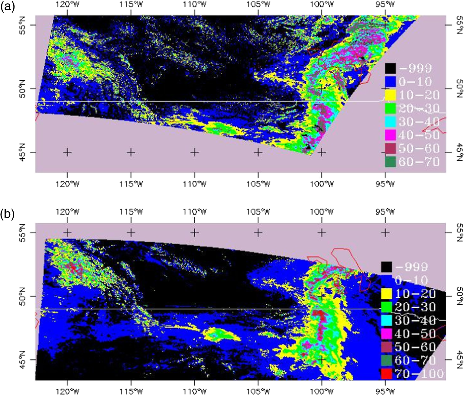
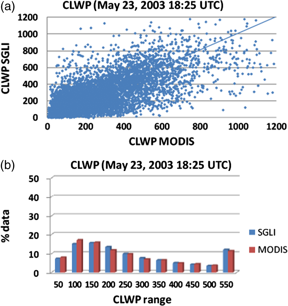
1.IntroductionEarth observation satellites missions, such as the Aqua/Advanced Microwave Scanning Radiometer for EOS (Aqua/AMSR-E), the Global Change Observation Mission-Water/Advanced Microwave Scanning Radiometer 2 (GCOM-W/AMSR2), the Terra- and Aqua-Moderate Resolution Imaging Spectroradiometer (Terra- or Aqua-MODIS), the National Oceanic and Atmospheric Administration/Advanced Very-High-Resolution Radiometer (NOAA-AVHRR), the ENVIronmental SATellite-MEdium Resolution Imaging Spectrometer (ENVISAT-MERIS) as well as the future GCOM-C/SGLI,1–3 are expected to monitor continuously various atmospheric constituents and to contribute to the development of useful geophysical products with high accuracy and reliability to be considered as “climate data records.”4 As the 15-year global environmental change monitoring mission5 of the NASA’s Earth Observing System (EOS) composed mainly of Terra and Aqua satellites6,7 is heading toward the end, there is a necessity for the development of follow-on missions with nearly similar or better spectral and spatial coverage, higher-sensor accuracy, and compatible channels (allowing for better connection between long-term data series). These qualities are expected from the promising GCOM-C/SGLI satellite mission [launch by the Japan Aerospace Exploration Agency (JAXA) expected around 2015 to 2016]. The primary objectives of the GCOM-C/SGLI satellite are not only to monitor long-term climate change, but also to improve the understanding of the Earth’s radiation budget and the carbon/hydrologic cycle mechanism.8 This satellite offers new opportunities in the analyses of global climate phenomena, and an appropriate transition to next generation sensors and satellites, thanks to the high-spatial resolution of its optical sensor, the SGLI (250 m for most of the channels), and the existence of both polarized and nonpolarized channels. Weather patterns around the globe have been changing rapidly in recent years. The increasing frequency of these changes has been mostly attributed to the temperature rise, the frequency of severe storms, drought, and precipitation.9–13 Due to these effects on climatic change, greater monitoring capacities are needed from actual and future Earth observation satellites’ sensors. Highly accurate algorithms that are used to transform these observations to physically meaningful quantities (geophysical properties) are also necessary. As customary, geophysical properties’ retrievals algorithms, at the prelaunch phase of satellites, are evaluated against other compatible satellites or field products,7,14–16 in order to assess the capacity of these algorithms to produce good quality data. The present study aims to conduct such an evaluation for the GCOM-C/SGLI prelaunch phase cloud properties algorithm. The performance of this algorithm (integrating spectral channels’ characteristics and response functions of the GCOM-C/SGLI satellite) is evaluated through a comparison against the MODIS algorithm, and then the accuracy targets of the new satellite mission are evaluated. Radiances and geometrical parameters from the Advanced Earth Observation Satellite-II/Global Imager (ADEOS-II/GLI), precursor of the GCOM-C/SGLI, serve as input data for the implementation of the cloud algorithm evaluated in this article. Spatially and near-timely matching () scenes to those of Terra-MODIS at various representative land and ocean areas of the globe during the year 2003 are selected as tests sites for this article. Among the parameters retrieved by the GCOM-C/SGLI algorithm, three direct cloud properties [the cloud optical thickness (COT), cloud particle effective radius (CLER), and cloud top temperature (CTT)] and one indirect property [the cloud liquid water path (CLWP)] are examined for the study. The output data obtained are compared with those of the MODIS sensor. The differences between the two sets of products are analyzed in terms of bias (differences MODIS-GCOM-C/SGLI) and root-mean square error (RMSE) of the GCOM-C/SGLI against MODIS. These results are then evaluated against the accuracy targets of the GCOM-C/SGLI mission. Finally, the major factors driving the discrepancies between the GCOM-C/SGLI and the MODIS products on one hand and the mission accuracy targets on the other hand are discussed, and possible remedies are evoked. The plan adopted to conduct this work is: following this “Introduction” section, Sec. 2 describes the characteristics of the GCOM-C/SGLI satellite and Sec. 3 provides some details about the algorithms examined in the article. Section 4 shows the performance tests results conducted on the GCOM-C/SGLI algorithm against the MODIS algorithm at various areas of the globe. Section 5 examines the degree of reliability of the products obtained relative to the accuracy target of the GCOM-C/SGLI products. Section 6 discusses possible reasons of the discrepancies between the two satellites’ products and the sensitivity of the GCOM-C/SGLI retrievals to the major assumptions made in the retrieval algorithm. Section 7 summarizes and concludes the study. 2.GCOM-C/SGLI SatelliteThe GCOM-C/SGLI is a part of two-component project, named GCOM. The other component of this project, the GCOM-W (GCOM-Water) satellite, was launched in May 2012. As stated earlier, the primary objective of the GCOM-C/SGLI satellite is to monitor long-term climate change and help to improve the understanding of the Earth’s radiation budget and the carbon/hydrologic cycle mechanism. For the entire mission, three series of satellites are expected to be launched for every 5-year period with a year of overlap interval between the series. Each satellite’s minimum lifetime is 5 years. The total observation period is 13 years. The satellite will fly on a sun-synchronous orbit at an altitude of 798 km with a descending local time . The optical sensor, the SGLI [Fig. 1(a)] carried by the satellite, has two components: the visible and near-infrared (SGLI-VNR) radiometer and the infrared (IR) scanner (SGLI-IRS). These components have a total of 19 channels [Fig. 1(b)]. The first component, the SGLI-VNR, is composed of 13 channels: 11 nonpolarization nadir view channels of 250-m spatial resolution and a swath of 1150 km and 2 polarization/along-track slant view channels having a spatial resolution of 250 m and a swath also of 1150 km. The second component, the SGLI-IRS, has six channels: four shortwave IR with a spatial resolution of and a swath of 1400 km and two thermal IR channels with a spatial resolution of 500 m and a swath of 1400 km. The GCOM-C/SGLI cloud algorithm examined in this article uses three channels belonging to the same component (the SGLI-IRS) for the retrieval of the cloud properties. Further details about the satellite mission are available at http://suzaku.eorc.jaxa.jp/GCOM_C/w_gcomc/whats_c.html. 3.Characteristics of the GCOM-C/SGLI and Terra-MODIS Cloud Properties Algorithms3.1.GCOM-C/SGLI AlgorithmThe cloud properties algorithm used for the GCOM-C/SGLI is named the Comprehensive Analysis System for Cloud Optical Measurement (CAPCOM). The algorithm is an enhanced version of the solar reflectance method algorithm initially used for the NOAA AVHRR data analysis.17 It is adjusted to the specific spectral channel characteristics and response functions of the GCOM-C/SGLI. During the prelaunch phase of this satellite mission, areal tests are conducted on various algorithms (among which, the cloud properties’ algorithm), to evaluate their performance. Based on these tests, the capacity of the algorithms to produce quality data that fulfill the satellite target accuracies is assessed. The input data for the implementation of this algorithm are radiances and geometry data of the ADEOS-II/GLI satellite (precursor of the GCOM-C/SGLI). The theoretical basis of the algorithm2 and other related information are summarized below. The algorithm uses radiances of three channels: a nonabsorption band (1.05 μm), an absorption band (2.21 μm preferentially used here compared with the 1.65 μm also available), and a thermal band (10.8 μm). It simultaneously retrieves the COT at 0.5-μm wavelength and the CLER using the combination of 1.05 and 2.21-μm wavelengths, as these bands primarily depend on the COT and the effective particle radius, respectively. The other input data needed for the retrievals are a cloud detection mask, ancillary data consisting of the surface albedo at the 1.05 μm and bands, the surface temperature, the atmospheric temperature, water vapor, and height profiles (from the Japan Meteorological Agency re-analysis data). The retrieval process starts with the determination of the CTT. This parameter is used to locate the position of the cloud prior to the application of atmospheric and surface corrections (using ancillary data from thermal and water vapor profiles and surface albedo) on nonabsorption and absorption channels. These correction data are then used for the final retrieval of the other parameters, among which are the COT, CLER, and CLWP. One of the specificities of this algorithm is the use for the entire retrieval process of three bands belonging to the same sensor component, i.e., the SGLI-IRS (this is supposed to help to avoid errors related to pixel-pixel mis-registration between channels of different sensor components), in contrast to MODIS where the channels used belong to at least two sensor components. As in most of the algorithms, such as those of the GCOM-C/SGLI or MODIS, geophysical properties (COT and CLER) retrievals are typically solved by comparing the measured reflectances with entries in a lookup table (LUT) and by searching for the combination of COT and CLER that gives the best fit.7 The first property to be retrieved in the GCOM-C/SGLI algorithm is the CTT. It is obtained through the infrared window method using atmospherically corrected brightness temperatures at 10.8 μm. For all the cloud properties examined in this article, four LUTs are used under a water cloud scheme for the retrievals: cloud-reflected radiance in bands 1.05 and 1.65 μm, transmissivities and reflectivity in bands 1.05 and 2.2 μm, respectively, and band 10.8-μm transmissivity. The grid system of the LUTs is composed of the equivalent water vapor amount of above cloud, the cloud layer, and below cloud, and then the cloud top height and cloud geometrical thickness, the satellite zenith, solar zenith, relative azimuth angles, and the simulated COT and CLER. To build these LUTs simulating the satellite signal, an efficient radiative transfer scheme18–20 is used. A log-normal size distribution, function of the particle radius with a mode radius related to the effective particle radius as , a log-standard deviation of the size distribution for marine stratocumulus clouds (), and a Lambert surface (underlying surface) are assumed for the computations. Based on the radiative transfer theory for parallel-plane layers with an underlying Lambert surface, the unexpected radiation components, such as the solar radiation reflected by the ground surface and the thermal radiation emitted from the cloud layer and the ground surface, are removed from the satellite-received radiance in order to decouple the radiation component reflected by the cloud layer. The solar radiation reflected by the ground is removed through the use of the ground albedo data. When the removed radiation significantly dominates over the signal, the algorithm’s main iteration may not converge. This mainly occurs at optically thin clouds. When that is the case, the analysis does not go further and is consequently cancelled. Multiple reflections between the ground surface and the upper layer are taken into consideration, though their effect may be negligible, especially for optically thin clouds and ground surfaces with low reflectance. But, with optically thick clouds and large values of ground albedo, the effect is relatively large at visible wavelengths. 3.2.MODIS AlgorithmIn contrast with the GCOM-C/SGLI cloud algorithm, where all the retrievals are made from a single program, the MODIS retrievals are obtained through two algorithms: the optical thickness, effective particle radius, and thermodynamic phase algorithm (MOD05) for the COT and CLER retrievals,7 and the cloud top properties and thermodynamic phase algorithm21 for the retrievals of the CTT, the cloud top pressure (CTP), etc. Below is a summary description of these algorithms, as extracted from their respective algorithm theoretical-basis documents (ATBD). 3.2.1.MODIS cloud optical properties algorithmThe channels used for the MODIS cloud optical properties algorithm (MOD05) are the visible (0.645-μm over land, substituted by 0.858 and 1.240 μm over ocean and bright snow/sea ice surfaces, respectively) and near-infrared (1.64, or 2.13, or 3.75 μm). The CLER retrieval is mainly based on the 2.13-μm band in conjunction with a nonabsorbing visible band. The 1.64- or 3.75-μm bands may also be used for the CLER retrieval, each in conjunction with a corresponding visible band. In optically thick conditions, the COT and the CLER can be determined nearly independently, and thus, measurement errors in one band have little impact on the cloud optical property determined primarily by the other band. The MODIS level-1B calibrated radiance (MOD02) of the channels evoked above and geolocation fields (MOD03) are the basic inputs for the COT and the CLER retrievals. Seven additional inputs or ancillary datasets are needed (CTP and CTT, cloud mask, land surface temperature, sea surface temperature, atmosphere temperature profile, atmosphere moisture profile, and surface spectral albedo). In addition to the usual table lookup approach, the MODIS cloud optical properties algorithm utilizes an interpolation and asymptotic theory to fulfill the retrieval task, where appropriate.7 The application of the asymptotic theory of optically thick layers helps the computation of the reflection function for a given value of COT, CLER, and ground albedo to be determined efficiently and accurately. It thereby reduces the size of the LUTs required. The steps followed by the retrieval process of this algorithm are: first, the cloud mask information is read as it determines whether a given pixel is cloudy or clear. Then, the ancillary data subroutines are called, which is followed by the reading of Level-1B data (MOD02_1 km) and geolocation fields (MOD03_L1A). Information about the viewing geometry (satellite, solar zenith angles, and the relative azimuth angle) is also obtained at this stage. Atmospheric corrections (Rayleigh, water vapor, and other absorbing gases) to the radiance data are applied. Then the cloud property retrieval, using LUT libraries under a water cloud scheme (for this article), is made. As in the case of the GCOM-C/SGLI algorithm, the COT and the CLER are obtained through the comparison of the measured reflectances with entries in a LUT and the search for the combination of COT and CLER that gives the best fit. Output results are stored as MOD06 data products. As in the GCOM-C/SGLI algorithm, the reflected intensity field of the LUTs is computed from a radiative transfer model. Among the assumptions used in these computations, a variety of optical constants for liquid water clouds (e.g., separate complex refractive indices for different wavelengths ranges: , , and ); a natural log-normal size distribution for water droplets with an effective variance . MODIS radiances are influenced by atmospheric (molecular) absorption, the presence of clouds and/or aerosols type(s), and surface properties. Corrections of these factors are necessary to obtain the appropriate cloud TOA satellite radiances that are used against the LUT. In this process, the Rayleigh scattering in the atmosphere above the cloud is first treated. This scattering primarily affects the COT retrieval, since the Rayleigh optical thickness in the near-infrared is negligible. An iterative method is used for effectively removing Rayleigh scattering contributions from the measured intensity signal in the COT retrievals.7 Contributions of direct Rayleigh single scattering without reflection from the cloud and contributions of single interactions between air molecules and clouds are removed from the sensor-measured reflection function. Next, the influence of the surface reflectance on satellite-measured cloud radiances is corrected. The gaseous atmosphere (transmission and/or emission phenomena) impact is also corrected through the use of the correlated -distribution code.22 The thermal emission from the atmosphere above the cloud is usually of second-order importance, which contributes only a few percent to the total intensity. The atmospheric transmission to cloud top, direct plus diffuse, is likely to be about 90% to 95% for most of the bands, which causes a minimum of about a 10% reduction in solar-reflected signal if no atmospheric correction is taken into account.7 3.2.2.MODIS cloud top physical properties algorithmThe cloud top properties algorithm uses the following thermal region bands: 8.55, 11.03, 12.02, 13.335, 13.635, 13.935, and 14.235 μm, to retrieve the CTT, CTP, cloud thermodynamic phase, and cloud cover.21 The MODIS cloud top properties algorithm is described in its ATBD.21 The algorithm uses a -slicing method that corrects for possible cloud semi-transparency, to generate the CTT and the CTP at resolution (resolution enabling a signal-to-noise ratio enhancement). This technique is based on the observation that the atmosphere becomes more opaque due to absorption as the wavelength increases from 13.3 to 15 μm, and thereby causes radiances obtained from these spectral bands to be sensitive to a different layer in the atmosphere. The slicing is the most effective for the analysis of mid- to high-level clouds, especially for semi-transparent high clouds such as cirrus. In this retrieval process, the MODIS CTP and effective cloud amount (i.e., cloud fraction multiplied by cloud emittance) are first determined using radiances-measured spectral bands located within the broad 15-μm absorption region. One constraint to the use of the 15-μm bands is that the cloud signal becomes comparable with the instrument noise for optically thin clouds and for clouds occurring in the lowest 3 km of the atmosphere. When low clouds are present, the infrared window channel (11.03 μm) data are used to infer the CTT; and then, via model analysis, the CTP and the height are determined. In this infrared window channel process, the MODIS observed 11.03-μm brightness temperature (BT11) is compared with a corresponding brightness temperature profile derived from the gridded model product of the National Center of Environmental Prediction (NCEP) to infer a cloud top pressure, assuming the cloud emissivity to be unity. In brief, clouds are assigned a cloud top pressure either by or by infrared window calculations. Prior to all these treatments, cloud top properties data are corrected for zenith angle to minimize the impact of the increased path length through the atmosphere of radiation upwelling to the satellite; in general, the retrievals obtained are considered to be reliable for satellite viewing angles of less than 32 deg.21 4.Capacity Tests for the GCOM-C/SGLI AlgorithmThe potential performance of the cloud algorithm used for the derivation of the cloud geophysical properties of the GCOM-C/SGLI satellite is conducted through a series of areal global evaluation tests. The quality of the products obtained is measured against the accuracy targets of the satellite mission. The tests conducted consist of comparing cloud properties retrieved from this algorithm and those of a spectrally compatible satellite, Terra-MODIS. Three direct parameters retrieved by this algorithm (the COT, CLER, and CTT) and an indirect parameter (the CLWP) are the selected cloud properties. Calibrated radiances of the GCOM-C/SGLI satellite precursor, the ADEOS-II/GLI, are used as input data for the implementation of the algorithm. Matching cloud scenes (geographically representative land and ocean areas of the globe) between the GCOM-C/SGLI and MODIS satellites are the selected tests sites. All the MODIS data used in these comparisons are version 5.1 products. 4.1.Cloud Top TemperatureIn cloud properties algorithms, such as the GCOM-C/SGLI or MODIS algorithm, the vertical position of the cloud along the troposphere is important for the determination of the magnitude of the atmospheric corrections to be applied on the initial TOA radiances. The determination of the position of the cloud is essentially based on the CTT data. As seen earlier, the CTT of the GCOM-C/SGLI is obtained based on the infrared window method, while that of MODIS is either derived from the slicing (high and middle clouds) or from the infrared window method (low clouds). Figure 2 shows the CTT retrieved from cloud scenes of May 23, 2003, in North America (between Canada and the USA) for the GCOM-C/SGLI and the MODIS algorithms. This figure shows that in cold cloud areas, the GCOM-C/SGLI has higher CTT values than Terra-MODIS (e.g., the relatively large and nearly vertical cloud band at the right of the images where MODIS shows a larger extension of temperatures of the range than GCOM-C/SGLI). At warm cloud areas, MODIS clouds tend to be warmer than those of the GCOM-C/SGLI (e.g., above 50°N at the left of the scenes). Figure 3 represents the scatter plot [Fig. 3(a)] of the CTT between MODIS and GCOM-C/SGLI, and then the separate frequency histogram distributions [Fig. 3(b)] of the datasets of the satellites. These graphs confirm the tendencies noticed with the CTT comparison images, i.e., the GCOM-C/SGLI is systematically overestimated (compared with Terra-MODIS) in cold to relatively warm clouds. This positive bias of GCOM-C/SGLI CTT gets larger as we move toward mid-thermal clouds, i.e., at MODIS CTT near 245 to 250 K. A slightly negative bias occurs at warm clouds as the MODIS CTT tends to have higher CTT than that of the GCOM-C/SGLI. The frequency distribution histogram related shows that MODIS has a higher frequency of cold clouds () and very warm clouds () than the GCOM-C/SGLI, while the latter shows gradually abundant mid-thermal to warm clouds. Fig. 2(a) Cloud top temperature (CTT) retrieved from North America by GCOM-C/SGLI SGLI (May 23, 2003, 18:25 UTC) and (b) Terra-MODIS (May 23, 2003, 18:10 UTC).  Fig. 3Scatter CTT diagram corresponding to Fig. 2 and showing the relation between the GCOM-C/SGLI and the Terra-MODIS (a); then, the frequency data distribution histogram of these individual datasets (b).  4.2.Cloud Optical ThicknessAfter the position of the cloud along the troposphere has been determined and the necessary atmospheric corrections on the nonabsorption and absorption signals are made, the COT is retrieved by matching the corrected cloud reflectances with the LUT reflectances. The present version of the GCOM-C/SGLI cloud algorithm determines the COT LUT in the range 0 to 70, while that of Terra-MODIS is in the range 0 to 100. Consequently, the quantitative comparison between the two algorithms will be limited to COT values equal or below 70. Figure 4 shows the COT retrievals from similar scenes as those used for Fig. 2. This figure shows that, in low COT areas, the GCOM-C/SGLI has thicker clouds than MODIS (e.g., left of the scenes’ areas and below 50°N latitude showing larger extension of clouds in the 0 to 10 COT range in the MODIS scene than that of GCOM-C/SGLI). This is also true in relatively thick cloud areas (e.g., the vertical cloud band at the right of the scenes shows a wider spread of large COT in the GCOM-C/SGLI scene than that of MODIS). Figure 5 is the scatter plot between the two algorithms [Fig. 5(a)] and the corresponding frequency distribution histogram of the individual datasets [Fig. 5(b)]. The scatter plot shows a good alignment of the data along the line between the two algorithms. However, the dispersion around this line tends to increase with the increase in COT. In general, there is an apparent overestimation of the COT at thin and relatively thick clouds of GCOM-C/SGLI against MODIS (also, there is a higher frequency of thin and very thick clouds in MODIS than GCOM-C/SGLI), while the latter seems to slightly dominate in very thick cloud areas (). Fig. 5Scatter diagram of the COT corresponding to images in Fig. 4 and showing the relation between the GCOM-C/SGLI and the Terra-MODIS (a) data; then, the individual datasets frequency distribution histogram (b).  4.3.Cloud Particle Effective RadiusThe CLER is simultaneously retrieved with the COT. This parameter is mostly a function of the absorption channels (1.6, 2.1, or 3.75 μm). It reflects the size of the cloud particles. Its upper limit in the present version of the GCOM-C/SGLI algorithm is 62 μm, while that of MODIS is 100 μm. The comparison between the two satellites will then be limited to CLER values below 62 μm. Figure 6 shows this comparison. The visual matching is mostly satisfactory with nearly similar variations of CLER observed between the images. However, in small particle-dominated areas, the GCOM-C/SGLI tends to show lower CLER than Terra-MODIS (e.g., below 50°N latitude and the corner between 105°W and 110°W longitude, and then 52° latitude and around 105°W longitude). At large CLER areas, differences between the two algorithms’ retrievals are hardly apparent. The good match between the retrieval images is also reflected by the graphs of Fig. 7, where the scatter plot [Fig. 7(a)] between the two retrieval datasets and the frequency distribution histograms [Fig. 7(b)] are presented. In the scatter plot, a good alignment of the two datasets along their line is clearly visible and only few data show large deviations from that line. The distribution histogram shows that in the lowest range data (), the GCOM-C/SGLI has a larger data frequency than the MODIS. At mid-ranges, MODIS slightly dominates and at high ranges the frequency seems to be nearly similar. Around the line of the scatter plot between the two satellites, some of the GCOM-C/SGLI data show a constant value (). This happens because of the difficulties of the iteration method to properly derive the CLER of these clouds; therefore, the radius is approximated to a fixed value of 9.0. Fig. 7Scatter diagram of the CLER corresponding to Fig. 6 and showing the relation between the GCOM-C/SGLI and the Terra-MODIS (a); then, the related individual datasets distribution histogram (b).  4.4.Cloud Liquid Water PathThe CLWP, expressed in , represents the total amount of liquid water along a cloud column. It is obtained by combining the COT and CLER through the equation: where is the liquid water density.Figure 8 presents the CLWP scatter plot between the GCOM-C/SGLI and the MODIS and the individual CLWP datasets’ frequency distribution histograms. The figure shows how many of the deviations of the individual parameters of COT and CLER cancel out when combined to form the CLWP. This leads to a very good correlation between the satellites’ retrievals. Also, the frequency distribution of the two datasets is very much even along the CLWP ranges. 5.GCOM-C/SGLI Target AccuraciesBefore the launch of Earth observation satellite missions, there are usually some expectations about the degree of accuracy to be attained by direct and indirect products of the satellite. This accuracy depends not only on the sensor accuracy, but also on the reliability of the algorithms used to obtain the satellite-derived products. For the GCOM-C/SGLI satellite mission, the prelaunch phase accuracy targets for the cloud properties examined in this article, expressed as root-mean square error (RMSE) directly (for the CTT) or indirectly as RMSE% (for the COT, CLER, and CLWP), against MODIS are: 1.5 K for the CTT of a cloud at sea level (or 3.0 K above sea level), 50% for both the COT and CLER, and 100% for the CLWP. One of the aims of this article is to assess the capacity of the GCOM-C/SGLI cloud algorithm to produce data that satisfy the accuracy targets of the satellite mission. To verify this capacity, the GCOM-C/SGLI RMSE or RMSE% against MODIS calculated from the average of matching scenes’ values (several days during the period May 2003 to October 2003) at various representative areas of the globe are evaluated with the corresponding product target accuracy of the mission (Fig. 9). Fig. 9Average coincident scenes (several days of the period May 2003 to October 2003) comparison between the two algorithms for the CTT, COT, CLER, and CLWP parameters at various representative areas of the Globe; the corresponding RMSE (CTT) or RMSE% (COT, CLER, and CLWP); then, the satellite mission target accuracy (green vertical line).  First, let us look at the CTT. Though there seem to be a reasonably good alignment between the two satellites retrievals, the increasingly negative bias as we move toward mid-thermal clouds strongly increases the RMSE. The values obtained are generally beyond the accuracy target of the satellite mission. The largest RMSEs are found in equatorial forest areas. For the COT, the RMSE% is generally slightly higher than the target accuracy of the satellite mission. Besides there is a regular alignment and nearly even dispersion around the line between the GCOM-C/SGLI and the MODIS. Similar alignment patterns were noticed in other areas of the globe. For all the areas examined, the RMSE% is mostly between 55% and 65%. However, larger deviations from the mission accuracy target occur above forest (West Africa, Amazon) or desert (Sahara). These areas, located around the equator, have generally high occurrences of cirrus clouds. The CLER RMSE% is mostly within the target accuracy of the mission (the majority of the regions show values below 50% RMSE). As in the previous case, the largest RMSEs (%) tend to occur in forest areas (e.g., the North Amazon, where the value is nearly twice the target accuracy). For the CLWP, and as noticed before, some of the errors in the COT and the CLER retrievals tend to somehow cancel out. As a result, there is a better alignment (than in the cases of COT and CLER) along the line between the satellite datasets (Fig. 8). Similar patterns were seen in other areas of the globe. The RMSE% in nearly all regions is consequently below the accuracy target () of the satellite mission. Here also, forests areas show lower accuracies than other areas. 6.Interpretation of the Tests Results6.1.Discrepancies Between the RetrievalsIn the previous sections, the results of the GCOM-C/SGLI cloud algorithm performance tests were presented. In these tests, cloud retrievals from this new satellite cloud algorithm were evaluated through a comparison of these retrievals with MODIS cloud products. Also, the capacity of the algorithm to produce data that fulfill the accuracy targets of the GCOM-C/SGLI mission was assessed. The first parameter analyzed was the CTT. It showed large RMSE, particularly acute around mid-thermal clouds. This was the result of the GCOM-C/SGLI CTT systematic overestimation (compared with MODIS) in virtually all representative areas of the globe. The COT showed good alignment and nearly equal dispersion around the line, but RMSE% is slightly beyond the satellite mission accuracy target. The CLER showed better results than the COT as the accuracy targets were met in most of the cases. However, mid-CLER ranges seemed generally overestimated. This contributed to increase the average CLER values of the GCOM-C/SGLI against MODIS. To understand all these differences, we will examine the effects of the uncertainties in the cloud type interpretation, the cloud thermal properties, the solar and satellite geometries, etc., on these parameters. First, the effects of the uncertainty in the cloud-type interpretation on the cloud retrievals are examined. For this purpose, a simple cloud-type classification, using the split-window channels’ differences,23 i.e., the brightness temperature difference between the 11 and 12 μm (BT11—BT12) channels against the brightness temperature at the 11 μm (BT11), is used. The parameters involved in this classification (BT11 and BT12) are more independent in this article than the optical parameters used in other classifications. Four types of clouds are initially identified in this split-window channels’ classification: cirrus (Ci), dense cirrus (D-Ci), cumulonimbus (Cb), cumulus (Cu), and others or mixture of remaining clouds (Mix). For the purpose of our article, the cirrus clouds will be divided in two: cold cirrus or C-Ci () and warm cirrus or W-Ci (). Figure 10 shows the RMSE and bias at each cloud type for all the examined parameters. The CTT RMSE and bias are large not only in the Ci, but also in the Mix clouds, while the cumulonimbus (Cb) and the dense cirrus (D-Ci) clouds show the lowest RMSE (even below 1.5 or 3.0 K, which are, respectively, the satellite mission accuracy target at sea level and above) and bias. Between the Ci clouds, W-Ci clouds show the largest RMSE and bias. The Cu clouds have either higher or close RMSE and bias than Cb clouds. The trends noticed with the CTT are nearly similar with those of the COT, CLER, and CLWP, i.e., the lowest RMSE% are found with Cb and D-Ci, and the largest are seen with the W-Ci, then gradually lower values with the C-Ci and Cu. The areal comparison between the two algorithms showed that the RMSE or RMSE% for all parameters had the largest values consistently above forest areas. One major explanation of this situation is that most of the forest areas are around the equator, and this region has annually the highest frequency of cirrus clouds. These clouds have shown large discrepancies between the two examined satellites’ datasets. If we only compare the BTD of the clouds, it appears that the CTT, COT, and the CLER RMSE tend to increase with the increase of the BTD, at the upper end of which are the Ci clouds. The variation of the brightness temperature with respect to the wavenumber for the clouds is mainly due to multiple scattering and absorption processes inside the clouds.24 Because the emission is the dominant process in these thermal infrared wavelengths, the cloud absorption interpretation between the two algorithms may differ. To understand these processes, we will now examine the interpretation of the contribution of the cloud emission to the discrepancies between the algorithms. In the infrared wavelength, the radiance perceived by a sensor is a function of the radiation emitted from the target and the radiation emitted and absorbed by the intervening atmosphere, integrated over the response function of the sensor.15 The atmosphere radiation is treated by the atmospheric correction while the radiation of the target (cloud) is part of the cloud correction scheme. At a specific wavelength, the energy emitted by clouds is controlled by the average temperature of the cloud surface and the cloud emission properties.21 The cloud emission correction factor is mostly related to the cloud emissivity. When the emissivity at the 11 μm reaches 1, the clouds become black, and when it is lower, the clouds are considered as gray bodies. The change in the cloud effective emissivity, i.e., in cloud emissivity and/or cloud fraction, may have an important effect on the TOA radiance.21 For a given observed radiance, if the emissivity is overestimated, the cloud top pressure is also overestimated, putting it too low in the atmosphere.21 Figure 11 shows the comparison between the retrieved images of the CTT by the two algorithms and the cloud emissivity, and the cloud fraction maps obtained from MODIS. Areas where the GCOM-C/SGLI CTT is strongly higher than that of MODIS correspond to low emissivity areas, as shown by the red circles on the CTT and emissivity maps. There is no visible change in the cloud fraction accompanying the differences in CTT between the two satellites. A quantitative illustration of the relationship between the CTT discrepancies and the emissivity is shown in Fig. 12. The histogram of the emissivity variation with RMSE and bias shows a gradual decrease of the RMSE and bias with the increase of the emissivity: low cloud emissivity areas tend to correspond to the major areas of CTT discrepancies. The difference between the two algorithms is minimal (even lower than the GCOM-C target accuracy at sea level) for emissivity higher than 0.9, while at lower emissivity, the two algorithms gradually diverge. Based on these observations, we can separate the CTT values in two groups: large emissivity () and low emissivity () CTTs. The scatter plots between the two algorithms clearly show that low emissivity clouds are at the origin of the major differences between the algorithms. The large emissivity clouds match very well (strong correlation) and show very few differences between the two algorithms. The cloud emission method used by the GCOM-C/SGLI may, therefore, insufficiently correct the cloud brightness temperature data used for the CTT. It was also noticed that low emissivity clouds tend to show stronger discrepancies (though less pronounced than in the case of the CTT) than high emissivity clouds for the COT, CLER, and CLWP parameters. Fig. 11CTT maps of GCOM-C/SGLI (a) and Terra-MODIS (b); then, the corresponding cloud emissivity (c) and cloud fraction (d) from Terra-MODIS. The red circles represent areas where the GCOM-C/SGLI CTT is higher than that of Terra-MODIS and the emissivity changes related to those areas.  Fig. 12Cloud emissivity histogram variation with the CTT RMSE (a), the distribution of data used in histogram (b), and scatter plot of the CTT between the two algorithms for emissivity more and less than 0.9 (c and d, respectively).  The effects of the uncertainties of the solar and satellite geometries on the cloud properties discrepancies did show consistent patterns. These effects are therefore considered marginal. Besides the factors examined already, the CTT, COT, CLER, and CLWP RMSEs may be influenced by other factors as well. Among these factors we may cite, the uncertainties in the calibration of the absorption or nonabsorption channels, the cloud detection, the atmospheric correction, the ground surface reflection (based on the surface albedo) correction, the water vapor, and temperature profiles (ancillary data). These various factors are examined in the following sections through sensitivity tests analyses. 6.2.Sensitivity TestsMeasured and calculated radiances differ because of the cumulative effects of instrument noise, spectral response function errors, inadequate knowledge of the atmospheric and surface state, radiative model approximations, etc.7 In this section, we will try to examine the effect of perturbations of some of the cloud external assumptions on the retrievals. 6.2.1.Sensitivity to the ground surface reflectionThe radiation reflected by the Earth surface may impact the determination of the cloud reflection, especially the reflection of transmissive clouds, and therefore, the COT and CLER. In the algorithms examined in this article, the effect of the surface albedo is accounted for in the correction of the cloud reflectance. Results of sensitivity tests conducted on Siberia (land area) clouds to evaluate the effect of the inclusion or not of the ground surface reflection correction on the GCOM-C/SGLI COT and CLER retrievals show that the ground surface correction decreases the GCOM-C/SGLI retrieval RMSE% only by 1% and 0.04%, respectively, for COT and CLER. As may be expected, the highest changes occur with thin clouds made of cirrus (RMSE% decrease by 23% and 3%, respectively, for the COT and CLER, when ground surface corrections are made). 6.2.2.Sensitivity to channel 1.05- radiance uncertaintyThe 1.05-μm channel is the nonabsorption channel used by the GCOM-C/SGLI algorithm for the COT retrieval. The equivalent channel used by MODIS is channel 0.65 μm for land, 0.86 μm for ocean, or 1.240 μm for snow/ice. A 5% increase in the radiance of the 1.05-μm channel increases the RMSE% by 18% and 0.7% for COT and CLER, respectively. A 5% decrease in the radiance of the same channel leads to an RMSE% decrease of 1.8% and 1.6% for COT and CLER, respectively. Because the nonabsorption channels used by both satellites’ algorithms for the COT retrieval are different, it was worth examining the impact of these differences on the RMSE%. A simple way to do that is to compare, for example, the difference between the reflectance of similar channels with those of MODIS, i.e., 0.65 μm (land) or 0.86 μm (ocean) existing in the GCOM-C/SGLI and the 1.05-μm reflectance effectively used in the latter satellite algorithm. Figure 13 shows how these differences affect the RMSE%. As the reflectance difference increases, the COT RMSE% also increases. When there is almost no or very little difference between the two channels, the COT RMSE% is lower than the GCOM-C/SGLI target accuracy (). At larger reflectance differences, the RMSE% is also large and may be as high as 40%. Differences in the sensitivity of the 0.65 μm or 0.86 and 1.05-μm channels appear to explain some of the discrepancies between the COTs of the two algorithms. Fig. 13Differences between reflectance (R) values of the nonabsorption channels of the GCOM-C/SGLI (0.65 μm or 0.865 and 1.05 μm), i.e., R0.65–R1.05 for land and R0.865–R1.05 for ocean, against the GCOM-C/SGLI COT RMSE% and bias%. The 0.65 and 0.865 μm are equivalent to the channels used by Terra-MODIS in the COT retrievals. The land area is Siberia (a) and the ocean area is the South Atlantic (b).  6.2.3.Sensitivity to the 2.2- radiance uncertaintyThe 2.2-μm channel mostly governs the retrieval of the CLER. Calibration errors are expected to be within 2% for the Terra-MODIS 0.65, 1.64, and 2.13-μm bands; based on these values, the CLER expected uncertainty is within 1 to 3 μm for optically thick clouds.7 Perturbation tests conducted on the GCOM-C/SGLI 2.2-μm channel show that a 5% increase in the radiance of this channel leads only to a 2% decrease of CLER, while a decrease by 5% of the same radiances leads to an increase in the RMSE% by barely 1.4%. 6.2.4.Sensitivity to the 10.8- radiance uncertaintyThe 10.8-μm is mostly used to determine the CTT. This CTT will be then employed to obtain the position of the cloud. This position is used as preliminary input parameter for the proper retrieval of the COT and CLER. A 5% decrease in the channel 10.8-μm radiance leads to an RMSE CTT decrease of 0.03 K, a COT RMSE% increase of 6.7%, and a CLER RMSE% increase of 1.4%. A 5% increase of the same channel leads to a CTT RMSE increase of 1.2 K, COT RMSE% increase of 7%, and a CLER RMSE% decrease of 6%. 6.2.5.Sensitivity to the water vapor profile uncertaintyThe water vapor profile is used to correct the atmospheric absorption of the radiance transmitted to the cloud or reflected by the clouds. By increasing or decreasing the water vapor amount at each pressure level of the profile above Siberia, for example, by 20% and 40%, we obtained insignificant changes in COT and CLER RMSE% as well as the CTT RMSE. 6.2.6.Sensitivity to the temperature profile uncertaintyThe temperature profile is used not only for the atmospheric correction of the thermal radiation, but also to obtain the proper cloud top pressure and height, inferred by the comparison with the pressure and the height profiles. The decrease of the temperature profile at all pressure levels by 2 and 4 K leads to a decrease of the CTT RMSE by 0.8 and 1 K, respectively, an increase of the COT RMSE% by 12.4% and 12.3%, and a decrease of the CLER RMSE% by 9.6% and 9%. The increase of the same profile by 2 and 4 K still at all pressure levels leads to a slight increase of the CTT RMSE by 0.1 and 0.14 K, an increase by around 12% of the COT RMSE%, and a 12.4% and 12.7% increase of the CLER. 6.2.7.Sensitivity to the cloud detection uncertaintyThe pixels used in the implementation of the GCOM-C/SGLI cloud properties algorithms are selected following a cloud screening or cloud mask algorithm named CLAUDIA.25 The cloud mask allows the distinction of clouds following a clear sky probability scale ranging from 0 (100% cloud probability) to 1 (100% clear sky probability). Intermediate values have either a higher probability of clear sky (above 0.5) or a higher probability of cloud (below 0.5). All the values except “1” (100% clear sky probability) are used in the cloud properties determination. The comparison of these retrievals with those of MODIS shows that the cloud detection affects both the COT and the CLER. Figure 14 shows cloud retrievals above the Amazon forest, one of the forest areas that often showed large RMSE% of COT and CLER for all clouds, and 100% or less cloud probability. It appears clearly that the low-probability cloud pixels’ bad alignment along the line between the algorithms contribute to the increase of the RMSE% of both the COT and the CLER and the deterioration of the correlation between the datasets. No clear difference was noticed in the case of the CTT. The strongly overestimated CLER pixels which often blur the correlation between the two algorithms clearly belong to the low-probability clouds. When these clouds are removed, there is a good alignment along the line between the algorithms. The high RMSE% seen in COT and CLER are strongly due to the differences in the interpretation of the radiation of the low-probability clouds between the two algorithms. 7.ConclusionResults of the implementation of the GCOM-C/SGLI cloud algorithm were evaluated in this article through performance tests comparing the retrievals of this algorithm against those of a compatible satellite, MODIS, at various representative areas of the globe. Also, the capacity of the algorithm to fulfill the accuracy targets of the satellite mission was assessed. The analyses conducted showed that there was sufficient alignment in most global areas between the GCOM-C/SGLI and the MODIS products for the CTT, COT, CLER, and CLWP examined in the study. However, a large overestimation of the GCOM-C/SGLI CTT, mostly around mid-thermal clouds, strongly contribute to high-RMSE values obtained for this parameter as well as the deviation from the accuracy targets of the mission. In the areal comparison, forests areas were the most problematic, as the RMSE or RMSE% of all the parameters was larger than in other areas and often beyond the accuracy targets of the satellite mission. The differentiation of cloud types showed that cirrus clouds had the strongest discrepancies between the algorithms, and the study demonstrates that the discrepancies in these clouds largely contributed to the low accuracy noticed in forest areas. In the analysis of the CTT, it was shown that the main reason for the discrepancies with Terra-MODIS was the emissivity difference. In practically all regions, the GCOM-C/SGLI RMSE increased with the decrease of the cloud emissivity, which implies an insufficient correction for this parameter in the GCOM-C/SGLI algorithm. The COT and the CLER accuracy analysis revealed that among the most influential factors driving the discrepancies between the two algorithms, the cloud detection uncertainty related radiation, the nonabsorption channel sensitivity (for the COT), played a major role. Low-probability clouds degraded the correlation between the algorithms, while with pixels of 100% cloud probability, the dispersions along the line between the algorithms was dramatically reduced for both the CLER and COT. To correct the insufficient cloud emissivity of the GCOM-C/SGLI, a BTD emissivity retrieval method could be used, instead of a (channels not available in the GCOM-C/SGLI) method employed by MODIS for this effect. For the COT, the nonabsorption channels for land and ocean used by the MODIS algorithm exist in the GCOM-C/SGLI. ReferencesF. AiresC. Prigent,
“Toward a new generation of satellite surface products?,”
J. Geophys. Res., 111
(D22),
(2006). http://dx.doi.org/10.1029/2006JD007362 JGREA2 0148-0227 Google Scholar
T. Nakajimaet al.,
“Overview and science highlights of the ADEOS-II/GLI project,”
J. Remote Sens. Soc. Jpn., 29
(1), 11
–28
(2009). Google Scholar
J. R. Dimet al.,
“The recent state of the climate: driving components of cloud-type variability,”
J. Geophys. Res., 116 D11117
(2011). http://dx.doi.org/10.1029/2010JD014559 JGREA2 0148-0227 Google Scholar
B. A. Baumet al.,
“MODIS cloud-top property refinements for collection 6,”
J. Clim. Appl. Meteor., 51
(6), 1145
–1163
(2012). http://dx.doi.org/10.1175/JAMC-D-11-0203.1 JCAMEJ 0733-3021 Google Scholar
C. E. SchuelerW. L. Barnes,
“Next-generation MODIS for polar operational environmental satellites,”
J. Atmos. Oc. Tech., 15
(2), 430
–439
(1998). http://dx.doi.org/10.1175/1520-0426(1998)015<0430:NGMFPO>2.0.CO;2 JAOTES 0739-0572 Google Scholar
W. BarnesV. Salomonson,
“MODIS: a global image spectroradiometer for the Earth observing system,”
Crit. Rev. Opt. Sci. Technol., CR47 285
–307
(1993). CROTE2 1018-1997 Google Scholar
M. S. Kinget al.,
“Cloud retrieval algorithms for MODIS: optical thickness, effective particle radius, and thermodynamic phase,”
in Algorithm Theor. Basis Doc. ATBD MOD-05,
Google Scholar
J. R. DimT. Y. NakajimaT. Takamur,
“Performance and sensitivity tests of the future climate satellite GCOM-C/SGLI’s cloud algorithm,”
in Proc. CMOS/AMS Joint Meeting,
(2012). Google Scholar
P. R. FieldR. Wood,
“Precipitation and cloud structure in mid-latitude cyclones,”
J. Clim., 20 233
–254
(2007). http://dx.doi.org/10.1175/JCLI3998.1 JLCLEL 0894-8755 Google Scholar
S. DiasA. F. Maria,
“An increase in the number of tornado reports in Brazil,”
Weather Climate Soc., 3
(3), 209
–217
(2011). http://dx.doi.org/10.1175/2011WCAS1095.1 1948-8327 Google Scholar
M. J. Hoerlinget al.,
“On the increased frequency of mediterranean drought,”
J. Clim., 25
(6), 2146
–2161
(2012). http://dx.doi.org/10.1175/JCLI-D-11-00296.1 JLCLEL 0894-8755 Google Scholar
L. Cuoet al.,
“Climate change on the northern Tibetan plateau during 1957–2009: spatial patterns and possible mechanisms,”
J. Clim., 26
(1), 85
–109
(2013). http://dx.doi.org/10.1175/JCLI-D-11-00738.1 JLCLEL 0894-8755 Google Scholar
S. MorakG. C. HegerlN. Christidis,
“Detectable changes in the frequency of temperature extremes,”
J. Clim., 26
(5), 1561
–1574
(2013). http://dx.doi.org/10.1175/JCLI-D-11-00678.1 JLCLEL 0894-8755 Google Scholar
S. A. Ackermanet al.,
“Discriminating clear sky from clouds with MODIS,”
J. Geophys. Res., 103
(D24), 32141
–32157
(1998). http://dx.doi.org/10.1029/1998JD200032 JGREA2 0148-0227 Google Scholar
R. AlleyM. Jentoft-Nilsen,
“ASTER algorithm theoretical basis document for brightness temperature, version 3.0,”
Los Angeles
(1999). Google Scholar
D. K. HallG. A. RiggsV. Salomonson,
“Algorithm theoretical basis document (ATBD) for the MODIS snow and sea ice-mapping algorithms,”
(2001) http://modis.gsfc.nasa.gov/data/atbd/atbd_mod10.pdf Google Scholar
T. Y. NakajimaT. Nakajima,
“Wide-area determination of cloud microphysical properties from NOAA AVHRR measurements for FIRE and ASTEX regions,”
J. Atmos. Sci., 52
(23), 4043
–4059
(1995). http://dx.doi.org/10.1175/1520-0469(1995)052<4043:WADOCM>2.0.CO;2 JAHSAK 0022-4928 Google Scholar
T. NakajimaM. Tanaka,
“Matrix formulations for the transfer of solar radiation in a plane-parallel scattering atmosphere,”
J. Quant. Spectrosc. Radiat. Transf., 35
(1), 13
–21
(1986). http://dx.doi.org/10.1016/0022-4073(86)90088-9 JQSRAE 0022-4073 Google Scholar
T. NakajimaM. Tanaka,
“Algorithms for radiative intensity calculations in moderately thick atmospheres using a truncation approximation,”
J. Quant. Spectrosc. Radiat. Transf., 40
(1), 51
–69
(1988). http://dx.doi.org/10.1016/0022-4073(88)90031-3 JQSRAE 0022-4073 Google Scholar
K. Stamneset al.,
“Numerically stable algorithm for discrete-ordinate-method radiative transfer in multiple scattering and emitting layered media,”
Appl. Opt., 27
(12), 2502
–2509
(1988). http://dx.doi.org/10.1364/AO.27.002502 APOPAI 0003-6935 Google Scholar
W. P. MenzelR. A. FreyB. A. Baum,
“Cloud top properties and cloud phase algorithm theoretical basis document,”
in MODIS/MOD04 ATBD,
63 Google Scholar
D. P. Kratz,
“The correlated k-distribution technique as applied to the AVHRR channels,”
J. Quant. Spectrosc. Radiat. Transf., 53
(5), 501
–517
(1995). JQSRAE 0022-4073 Google Scholar
T. Inoue,
“A cloud type classification with NOAA 7 split-window measurements,”
J. Geophys. Res., 92
(D4), 3991
–4000
(1987). http://dx.doi.org/10.1029/JD092iD04p03991 JGREA2 0148-0227 Google Scholar
M. C. Wu,
“A method for remote sensing the emissivity, fractional cloud cover and cloud top temperature of high-level, thin clouds,”
J. Clim. Appl. Meteor., 26
(2), 225
–233
(1987). http://dx.doi.org/10.1175/1520-0450(1987)026<0225:AMFRST>2.0.CO;2 JCAMEJ 0733-3021 Google Scholar
H. IshidaT. Y. Nakajima,
“Development of an unbiased cloud detection algorithm for a spaceborne multispectral imager,”
J. Geophys. Res., 114 D07206
(2009). http://dx.doi.org/10.1029/2008JD010710. JGREA2 0148-0227 Google Scholar
BiographyJules R. Dim received his PhD in hydro-geophysics from the Center for Environmental Remote Sensing (CEReS) of Chiba University, Japan, in 2002. After working as postdoctoral fellow/researcher at Luleå Technical University in Sweden, then Hokkaido University and Chiba University in Japan, he joined the Japan Aerospace Exploration Agency (JAXA) in 2008. His research interests are atmospheric radiation, cloud and aerosols interactions with climate, validation of satellite derived clouds and aerosols properties with ground-based data, cloud inhomogeneity effects on satellite observations Takashi Y. Nakajima received his doctor of science degree in earth and planetary physics from the Center for Climate System Research (CCSR) of the University of Tokyo in 2002. He came to the Japan Aeorospace Exploration Agency in 1994 and moved to Tokai University in 2005. His present research themes are: remote sensing of clouds and aerosols, using visible and infrared multispectral radiometers; and the theory of light scattering by nonspherical particles. Tamio Takamura obtained his doctor of science degree in geophysics from Tohoku University in 1979. His major research is atmospheric physics. After working as a postdoctoral fellow for half a year, he joined the National Defense Academy as a faculty member in the Department of Mathematics and Physics. In 1986 to 1987, he worked at the University of Arizona as a visiting faculty member in atmospheric sciences. Since 1995, he has been in the Center for Environmental Remote Sensing (CEReS), Chiba University as professor. He is interested in atmospheric radiation, aerosol and cloud sciences. |