|
|
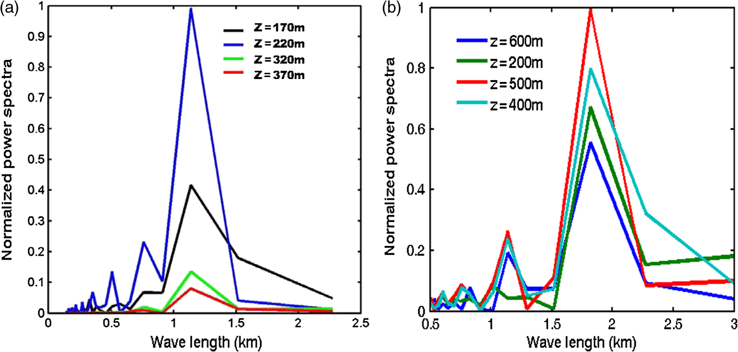
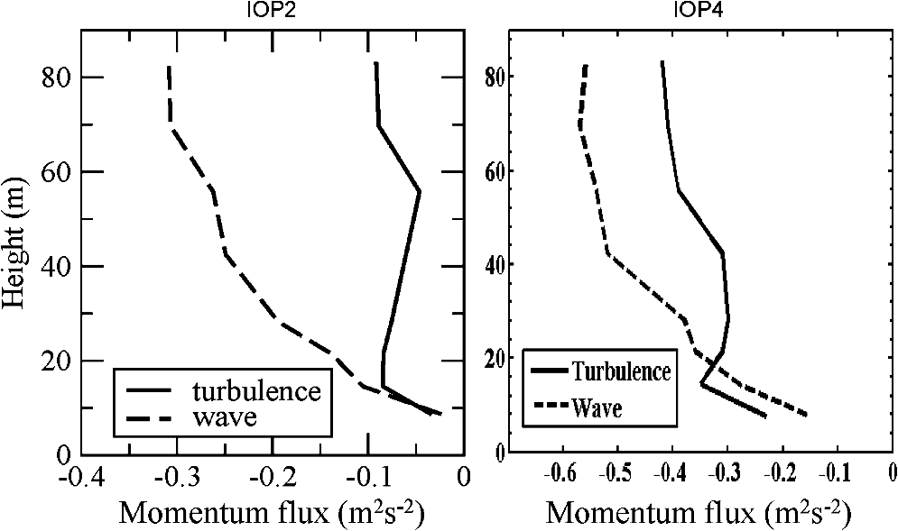
1.IntroductionThe nocturnal low-level jet (LLJ) is one of the frequently observed weather phenomena over land during clear night, weakly disturbed large weather conditions. According to Blackadar’s theory,1 the nocturnal LLJ is formed when the wind becomes decoupled from the surface due to the development of a stable surface layer and the air above the stable layer accelerates along the pressure gradient, and in addition, the Coriolis force induces an inertial oscillation that produces a greater speed than the geostrophic wind. There are numerous observational studies of nocturnal LLJ over many regions of the world,2–10 and they show that LLJ enhances the transport of momentum, heat, and moisture in the atmospheric boundary layer (ABL) and plays a role in deep convections. The climatology aspect of nocturnal LLJ over the Great Plains of the United States has been studied extensively by traditional radiosonde methods.2,7,9,10 Remote-sensing methods have also been used to investigate nocturnal LLJs. Using a Doppler wind lidar in the Cooperative Atmosphere-Surface Exchange Study 1999 (CASES-99), Banta et al.11 showed that nocturnal LLJs were common in undisturbed large weather conditions and often occur from 100 to several hundreds of meters above the ground level. Boundary layer wind data observed by Doppler wind lidars, radar wind profiler, and radiosonde over Oklahoma City (OKC) during the Joint Urban 2003 (JU2003) indicated that a strong southerly nocturnal LLJ dominated the ABL flow during the early morning hours of most of the intensive observation periods (IOPs).9,12–14 As shown in the continuous observations by the radar wind profilers,12 the LLJs start to develop right after sunset and afterward strengthen with time in a weak synoptic weather-forced condition. LLJs were well developed in 9 of 10 IOPs during JU2003. Nocturnal LLJs have a large influence on the underlying stable ABL and shear-generated turbulence.11,15–18 It acts as a momentum source in the stable ABL for the downward momentum transport, because the LLJ maximum is usually located several hundred meters above the ground surface. The LLJ not only produces greater turbulent kinetic energy (TKE) and enhances the turbulent mixing below the jet, but also transports the TKE from the jet’s maximum level downward to the ground surface when the lower part of ABL is stable.11,16 Banta et al.11 found that near-ground TKE was scaled well with a jet Richardson number in CASES-99 data, and the scaling relation was also evident in JU2003 data in the stable ABL.14 For similar reasons, nocturnal LLJ was also found to enhance the mixing and transporting of scalars (e.g., , , and water vapor) in the stable ABL.19,20 Wave motions are often associated with the nocturnal LLJs, which have strong wind shears and stable temperature stratifications. Wave motions produced by the LLJs have been studied in stable ABL at night times.21–24 It was concluded in these studies that wave breaking was one of the major causes of intermittent turbulence in the stable ABL. In fair weather conditions without frontal passage, the ABL has a typical diurnal cycle that is stable at night and convective during the daytime. The morning transition of the ABL from stable to convective starts right after sunrise. The ground surface absorption of the solar radiation produces the upward sensible heat flux and a convective boundary layer that grows quickly with a cap inversion layer on top. On the other hand, right after sunset, the ground surface cools and the sensible heat flux is reversed to downward, and a stable ABL starts to develop from ground up. While many observational studies have been carried out for waves in the nocturnal stable ABL, there are only few observational studies for the wave motions during the stable to convective transition period.25–27 In all three studies, the ABL wind in the mixed layer below the inversion layer did not have LLJs and the associated strong wind shear, but the momentum flux in the ABL did show the strong influence of the elevated inversion layer–generated wave motion. In our analysis of the JU2003 datasets, the nocturnal LLJ-generated gravity waves and strong wind shears were present below the cap inversion layer during the morning ABL transition hours. According to the linear stability theory,28 if the Richardson number of a stable layer of stratified flow is less than a critical value, instability will develop. Theoretical linear stability analysis has indicated the possibility of wave excitation in the cap inversion layer of an ABL.29 During JU2003, we have observed several episodes of gravity waves during the transition hours of ABL. In this article, we examine the gravity waves generated by LLJs during the transition hours of the ABL by analyzing the data from Doppler wind lidar, radar wind profiler, radiosonde, and sonic anemometers. The mechanism of the gravity wave generation by the LLJ is described for those cases during the ABL transition period. The wind signals from sonic anemometers on a tower are separated into waves and turbulence using a wavelet decomposition method, and the momentum fluxes due to these two components are computed. 2.InstrumentationThe data used in this study is from JU2003 observations. The JU2003 project, a cooperative undertaking to study turbulent transport and diffusion in urban ABLs, was conducted in OKC in late June through the end of July 2003.30 Besides numerous tracer samplers, a Doppler wind lidar, operated by the Army Research Laboratory (ARL), and a large number of sonic anemometers were deployed to monitor the wind field during the experiment. The Lawrence Livermore National Laboratory (LLNL) set up an 83-m high tower with eight sonic anemometers, which is located outside of the northern side of the central business district (CBD).9,31 The ARL Doppler lidar deployed in the project was a WindTracer® made by Coherent Technologies, Inc., in Lafayette, Colorado, and was designed specifically for ABL observations and research. Its laser wavelength and pulse energy is 2025 nm and 2.5 μJ laser, respectively. Furthermore, its pulse repetition frequency is 48 Hz, and the range gate varied from 66 to 71 m depending upon the dataset. The system measures range-gate resolved backscatter intensity and the Doppler radial velocity. The location of the ARL lidar is shown in Fig. 1, where the lidar was setup on top of a two story parking garage [global position system (GPS) coordinate: N 35° 28.385′, W 97° 30.266′, 20 m above ground]. Other relevant observations are radiosonde and radar wind profiler observations by Argonne National Laboratories (ANL) and Pacific Northwestern National Laboratory (PNNL). The ANL release site is located about 5.5 km north of the CBD, and the PNNL site is located about 0.8 km south of the CBD. During the IOPs, the radiosondes were released hourly to monitor atmospheric motions and variations. The ANL and PNNL also operated radar wind profilers at their sites, which provide hourly vertical wind profiles. Large amount of data were collected from the JU2003 project, and the data are stored and managed by Dugway Proving Ground. Fig. 1Aerial photograph showing the Army Research Laboratory (ARL) lidar site and Lawrence Livermore National Laboratory (LLNL) 83 m tower site, both denoted by two triangles. The central business district (CBD) of Oklahoma City (OKC) is located on the left portion of the photo in the yellow square. The yellow arrow line indicates the laser beams during IOP2 and IOP4 from the ARL lidar. The lidar signal range was 7 to 8 km, reaching out to the surrounding suburban area, much farther than shown in this figure. The Argonne National Laboratories (ANL) radiosonde release site is located about 5.5-km north of the CBD, and the Pacific Northwestern National Laboratory (PNNL) radiosonde release site is located about 0.8 km from the CBD; both locations are outside of the aerial photograph. 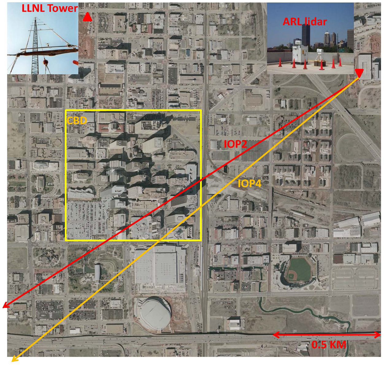 3.Data and Analysis3.1.Doppler Wind Lidar Images and Spectral AnalysisNocturnal LLJs were very common in the clear, undisturbed nights and early mornings during JU2003. LLJs appeared in 9 out of 10 IOPs, the lone exception being IOP1 which had convective disturbances due to a passing front.9–12 From wind profiler/rawinsonde observations12 and inspection of numerous lidar images,14 it appeared that the nocturnal LLJs start to form 1 to 2 h after sunset when the ground has cooled, causing a stable layer to develop just above the surface. The LLJs were fully formed around 10 PM local time and were generally strongest just before the sunrise, after which, they started to dissipate from the ground up during the transition from stable to convective boundary layer. Before the LLJs were totally destroyed by the underlying convective boundary layer growth, there was a period during which the atmospheric stability conditions are favorable in the cap inversion layer for shear-generated gravity waves. The gravity waves were fairly common during the transition period associated with the growing of the convective boundary layer. We have seen evidence of wavelike motion in many mornings during JU2003 from Doppler wind lidar images, but only two IOPs’ (IOP2 7/2/2003 and IOP4 7/9/2004) data were chosen for current analysis, since the complete dataset is available for these two cases. Figures 2 and 3 show the RHI (range-height-indicator) scan images of IOPs 2 and 4 at different times in which the wave motions appeared. The lidar scanning directions in these images were approximately parallel to the mean wind directions (see Fig. 1) at the LLJ levels with less than 10 deg of deviation according to mean wind profiles from the radiosondes. The elevation angle of the scan ranged from 0 to 45 deg. Horizontal wind speed was derived from the radial wind signal by dividing the cosine of the elevation angle, while assuming a two-dimensional flow at the jet level.14 A negative sign represents the wind direction that flows into the lidar in the RHI scanning plane. The gravity waves appeared to be nonlinear, because their wavelength depended on their distance from the lidar. The waves in the IOP2 were shorter in wavelength than that of IOP4, and the LLJ height in IOP4 was much higher than the heights in IOP2. In both cases, the layer above the wave motion, usually characterized as the residual layer from the previous day’s convective turbulence decay, had little wave signatures. Although the wavelengths and heights of the LLJ in those cases were different, they showed some similarity in distinct turbulent air motion near the ground surface below the wave. The gravity waves and turbulent motions appeared to have a strong interaction. A slightly elevated LLJ and wave motion over the urban area was observed in IOP2 cases. This is probably due to the lower altitude of the LLJ in the IOP2 and the urban heat island effect,14 which was able to reach this height and not the higher altitude of the LLJ in IOP4. As opposed to a nocturnal gravity wave observed when the entire boundary layer is stable,21,23 the wave did not display overturn or billows in IOP2 or IOP4. This is probably because the lower part of the boundary layer below the cap inversion layer was already in a neutral condition in these IOPs, which had a dissipative effect on the wave motion. Fig. 2Doppler wind lidar horizontal wind at different times during IOP2. The azimuth direction for the RHI scan was approximately parallel to wind direction (238 deg). In the figure, the lidar is located at (0, 0), and positive horizontal wind speeds indicate wind flow away from the lidar. 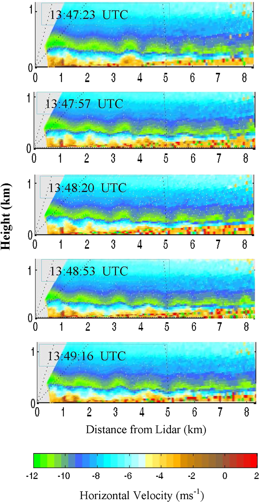 Fig. 3Doppler wind lidar horizontal wind at different times during IOP4. The azimuth of the RHI scan was approximately parallel to wind direction (230 deg).  Figure 4 shows the spectral analysis that was performed on the lidar horizontal wind speed for IOP2 and IOP4. These are the averaged power spectrum values of the five frames shown in Figs. 2 and 3 and normalized with the highest power spectra values from each scanning frame. The spectrum shows distinct peaks for the dominant average lengths for 1.1 and 1.8 km for IOP2 and IOP4, respectively. The spectral analysis indicated that the power spectrum is different at different heights for both of these cases, and the strongest spectra were at the heights of the LLJ maxima for both cases. The decay of wave motion above the LLJ maximum occurred more rapidly than below the LLJ maximum. By tracking the wave peaks in the lidar image, the wave phase speeds were estimated to be for IOP2 and for IOP4. 3.2.Radar Wind Profiler, Radiosonde, and Linear Atmospheric Stability AnalysisThe wave generation is determined by the mean atmospheric wind shear and temperature stratification. Figure 5 shows vertical profiles of horizontal wind and potential temperature before and after the wave motions for both IOP2 and IOP4. The potential temperature was measured by the ANL rawinsonde, while the horizontal winds were measured by the radar wind profiler since the radiosonde’s wind profiles did not have enough data points at altitudes below 200 m. Before the wave activity, the data shows that the strongest shear of the jet is located just below the jet nose or maxima, and the potential temperature profile indicated that a near-neutral stratification was present near the ground at the time. There was a strong stable stratification layer right below the height of the jet speed maximum, and this is where the gravity waves were produced. After the wave motion, the lower boundary layer temperature warmed and the wind profiles generally showed reduced wind maxima at the altitude of the LLJ. In addition, the stratification at the LLJ maxima reduced, and the LLJs moved higher than before the wave motion. The convective boundary layer grew significantly during the wave motion periods which also resulted in a well-mixed equilibrium state, as indicated by the wind and temperature profiles. Fig. 5Average wind and temperature profiles before (thick lines) and after (thin lines) gravity wave events for IOP2 and IOP4 measured by ANL radar wind profiler and radiosonde. 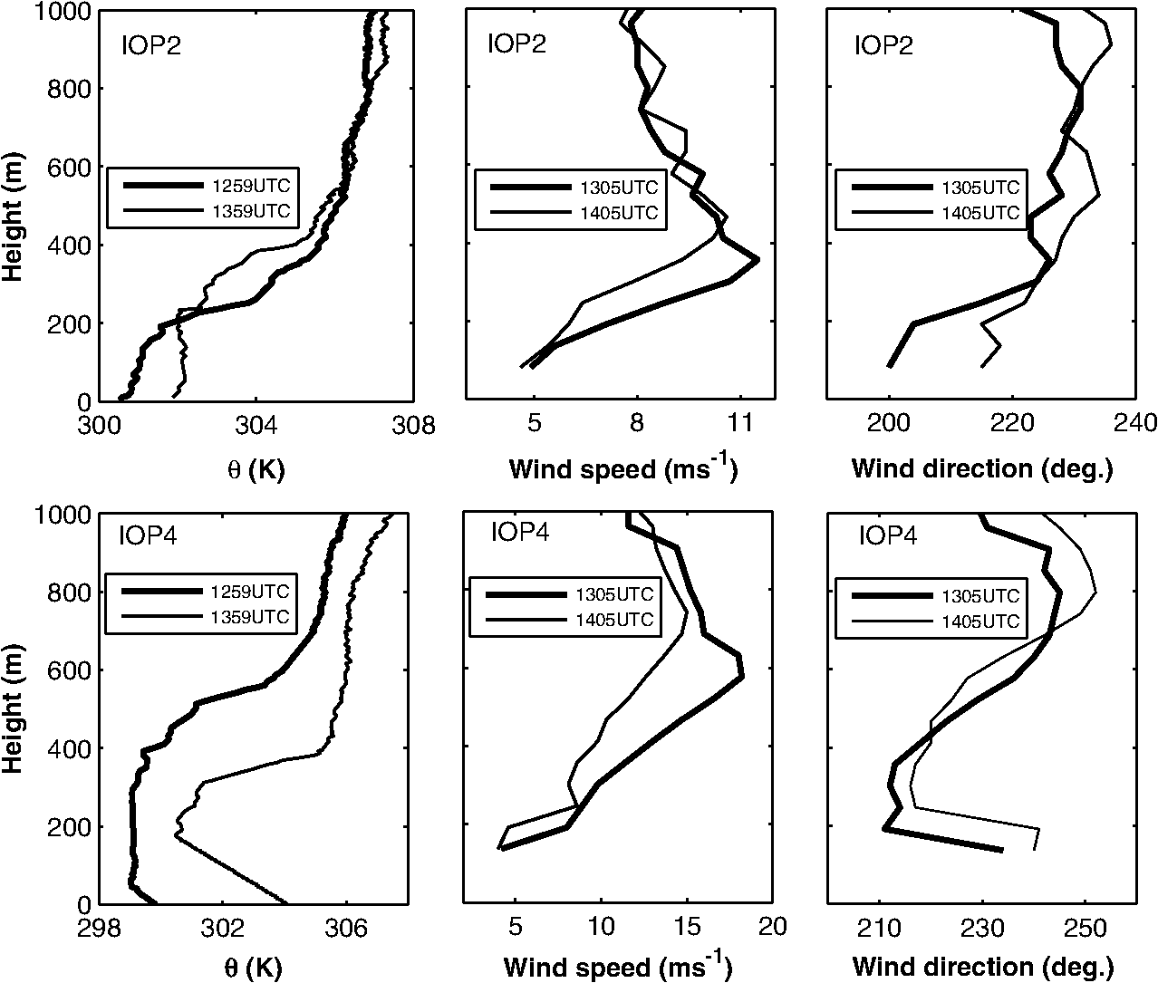 A linear stability analysis was carried out for these two wave events using the radiosonde and radar wind profiler data. Figure 6 shows the horizontal wind profiles from the radar wind profiler and temperature profiles from both the PNNL and the ANL sites. As similar temperature stratification and wind shear were observed in previous studies that have used standard linear stability analysis,29,27 we have used the basic theoretical conclusions resulting from these studies for the analysis that we perform. The PNNL and ANL data agreed reasonably well before the wave episodes, even though the two sites were about 6.3 km apart. Since the ANL data were more complete at the lower levels, the Brunt–Väisälä (or buoyancy) frequency () and gradient Richardson number () were computed from the ANL data as follows: where is the mean potential temperature, is the gravitational acceleration, and is the mean horizontal wind speed. is the upper frequency limit for the internal gravity waves,28,32 and is the atmospheric stability parameter determined by the mean temperature gradient and wind shear. The computation of and is very sensitive to temperature gradients and wind shear—a slight change of potential temperature and wind speed can cause a large change in these two parameters. The temperature profiles were smoothed using a running average, before they were used for the computation of the and parameters. For IOP2 [Figs. 6(a)–6(c)], indicates a slightly unstable condition below 0.15 km and almost neutral conditions from 0.15 km to the LLJ nose (0.35 km). Just below the LLJ nose, there is a stable layer where is slightly less than 0.25, which is the critical value for the development of instability according to the theoretical analysis of Miles and Howard.28 Below this value, the gravity wave appears. The critical can be greater than 0.25 in some conditions. According to Fernando,18 several laboratory results indicated that the critical can be as large as 1.0. Doppler lidar data (Fig. 2) indicated that the wave motion appeared in the cap inversion layer, but it was damped out above the LLJ. The vertical profiles for IOP4 [Figs. 6(d)–6(f)] show similar temperature and wind shear structure, but the stable cap layer was from 0.3 to 0.6 km above-ground level (AGL) which is thicker than the structures that appeared in IOP2. The value at this layer, whose altitude was approximately 0.4 km AGL, was near the critical value but slightly greater (0.5 to 0.6). The average buoyancy frequencies, , at the wave excitation layer is larger in the case of the IOP2 (0.035 Hz) than for IOP4 (0.022 Hz). In general, gravity waves have the highest when atmospheric temperature stratification is present. However, time series analysis of the sonic anemometer signal showed much lower frequency than the value calculated for , which indicates a very unstable mode for the wave frequency.Fig. 6Wind and temperature profiles at the PNNL and ANL sites and the computed Richardson number () and Brunt–Väisälä frequency () using the ANL data before the gravity episodes for IOP2 (a–c) and IOP4 (d–f).  The wavelength is very much related to the depth of the stratified shear layer. The typical wavelengths range from to , where is the depth of the stratified shear layer.28 Using the estimate of the stable cap layer depth from Fig. 6 from both IOP2 () and IOP4 () and the dominant wavelengths (Fig. 4, and 1.8 km for IOP2 and IOP4, respectively) from spectral analysis results, the relationship between the shear layer depth and the wavelength was established, to . This relation from the observational data agreed with the theoretical analysis. As the Doppler lidar wind data show (Figs. 2 and 3), the gravity waves are not quite linear, because they have slightly different wavelengths and amplitudes. This nonlinearity is expected in these two cases of ABL not only for the nonuniform atmospheric shear stratification, but also for the different ground surface conditions along the wave-propagation direction. The linear stability analysis gives a reasonably good prediction of the wave characteristics over a relatively uniform and flat terrain. Nonlinear variation and the intermittency of the wave characteristics in space and time cannot be described by the linear theory. 3.3.Separation of Wave and Turbulence Wind SignalsAlthough the gravity waves originated from the stable cap layer several hundred meters above the ground, the question to ask is how do they affect both the atmospheric momentum transport in the ABL below the cap and the overall ABL transition from stable to unstable conditions? To answer these questions, we will use data from eight sonic anemometers on the 83-m LLNL crane-tower.9,31 Sonic anemometer-observed wind signal time series are analyzed using a wavelet technique to characterize the wave impact on the vertical momentum fluxes. We chose to use the wavelet transform technique, because it is more appropriate than the Fourier transform for the nonstationary intermittent turbulence time series.33,34 In contrast to the Fourier transform, the wavelet analysis is performed locally in time domain by dilating or contracting a wavelet basis function. While both transforms conserve the energy in the physical space, the advantage of wavelet analysis over the Fourier transform is that it preserves the local information of a signal. The local wavelet transform is not affected by the behavior of the signal far away in the physical space. The temporal variation of a turbulent wind signal is especially important for understanding the interactions between nonstationary, spatially coherent wave structures and incoherent turbulence. Furthermore, use of orthogonal wavelet bases allows one to decompose and reconstruct a signal which is useful to separate the gravity waves and turbulence signals. For detailed general descriptions of the wavelet transform and its application in turbulence research, the readers are referred to monographs35 and general reviews.33,34 We only describe the basic wavelet analysis methods used in this research. The wavelet transformation coefficient of a function is an integral transformation defined as where is the wavelet basis function, is the scale parameter, and is the location parameter in the wavelet basis function ( and are time scale and time instance location, respectively, in this analysis). For the LLNL tower, the sonic anemometer data were discrete and collected with 10-Hz frequency; therefore, a discrete wavelet transform should be applied. For a discrete wavelet transformation, a dyadic scale and translation are used, i.e., and , the wavelet basis function can be written in the following discrete form: where and are the scale and location indexes, respectively.A turbulent wind signal can be decomposed into orthogonal wavelet series with the wavelet basis : where are the wavelet coefficients from the transformation. Since the wavelet basis functions are orthogonal, the wavelet coefficients can be computed from the inner product of the turbulent signal and its wavelet basisUsing the wavelet multiresolution analysis technique,36 the turbulent wind signals can be decomposed into the fine-scale turbulent and large-scale coherent parts. The wavelet decomposition produces a family of hierarchically organized signals. The choice of a suitable level for the hierarchy to separate the turbulence from the signal is largely dependent on the signal being analyzed. Howell and Mahrt37 have used the ratio of turbulence variance to total variance in the low-pass filtered signal to determine the level of the wavelet decomposition. In our analysis, we choose to use the recursive method by Farge et al.38 to separate the turbulent and wave parts from the signal. The wavelet basis function is the Symlets,35 which is an orthogonal function. In this algorithm, an optimal threshold is iteratively determined without any adjustable parameters. It has been proven to be very robust in the separation of the coherent large-scale and turbulence signals.38 Given a time series with discrete samples, we initially set , where represents the number of data points in the incoherent turbulent signals. A wavelet transform is performed to obtain the wavelet coefficient . The threshold (), a dependent variable of the wavelet coefficient , is estimated by A recursive loop () is entered after initialization. For the ’th iterative step, we count the number of wavelet coefficients less than , which gives a new , and then set and compute the new variance using the wavelet coefficient less than the , , and recomputed a new threshold for the next iteration, . Next, in an iterative fashion, we repeatedly set until . The final step is reconstructing the coherent signal using all wavelet coefficients greater than the threshold, , using Eq. (4). The difference between the original signal and the coherent signal is the turbulence signal. Before the wavelet analysis, the sonic , , signal was rotated in such a way that the mean wind is oriented along the direction. Since the wave observed during IOP2 and IOP4 are quasi two-dimensional, only and components are analyzed via the wavelet decomposition method. Furthermore, the mean wind speed was subtracted from the signal before the analysis. Figure 7 shows an example of wavelet decomposition of IOP4 sonic anemometer signals into three parts—the mean, the wave (∼), and the turbulent fluctuation (´) at . Fig. 7An example of wavelet decomposition of and wind components of sonic anemometer wind data at 83.2-m height during IOP4. It is decomposed into mean, wave (∼), and turbulent fluctuation (´) parts. 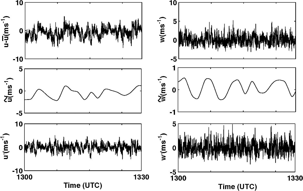 Figures 8 and 9 show the LLNL tower sonic anemometer-observed horizontal and vertical winds during IOP2 and IOP4 after a signal decomposition using the wavelet technique. The gravity waves generated by the LLJ at the inversion cap layer are measured in situ by the sonic anemometer and shown in the time series plots of Figs. 8 and 9. The wave motion appeared in both the horizontal and vertical wind signals which were in coherent, near-quadrature fluctuations with ahead of , which is a typical signature of wave motion. The wave motions were nonlinear with some variations of amplitude and period. Further inspection of the wave signals from the tower sonic anemometers indicated that the wave originated at higher levels with the lower level signals lagging behind. The wave signals at different levels also show a damping effect with smaller amplitudes in lower levels. Fig. 8Horizontal (a) and vertical (b) wind time series from LLNL tower sonic anemometers during IOP2. The signals are low-passed wave part of the wind using the wavelet separation technique. The heights of anemometers are labeled on the color-coded curves, applying for both panels. The signals are also transformed and plotted by adding a number, so the curves are readable.  Fig. 9Horizontal (a) and vertical (b) wind time series from LLNL tower sonic anemometers during IOP4. The signals are the low-pass-filtered part of the wind signal using the wavelet separation technique. The heights of anemometers are labeled on the color-coded curves. The signals are transformed and plotted by adding a number, so the curves are readable. 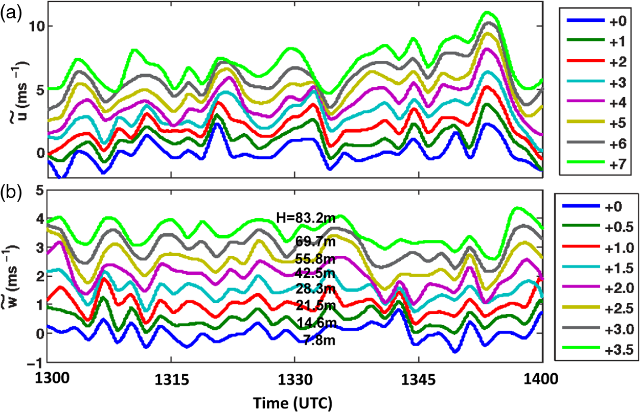 Gravity waves not only feed energy to small-scale turbulence through wave breaking and instabilities, but also directly contribute to the transport of momentum. Figure 10 shows that the wave momentum flux is 1.5 to 3 times greater than the turbulent momentum flux at higher levels and approaches it in magnitude near the ground surface. The negative sign indicates that wave momentum is transported to the ground and is absorbed by the ground surface. The higher momentum transport was transported downward by the wave momentum flux, which indicates the importance of the role that gravity waves play in the ABL transition from stable to unstable condition; namely, it accelerates the ABL transition toward the well-mixed equilibrium condition. 4.Summary and ConclusionsDoppler lidar RHI scans and in situ wind sensors have indicated that linear waves exist during the transition periods from stable to convective boundary layers in the morning hours of JU2003. For nondisturbed conditions, the LLJ was a dominant flow feature over OKC during the night to morning hours. The LLJ creates a large shear from jet maximum to ground. Temperature stratification was favorable during the boundary layer transition period, and during this time, the gradient Richardson number is reduced below the critical value of 0.25 and gravity waves are generated. The linear analysis indicates that it was plausible for the generation of the gravity waves in the stable stratified cap layer. The wind signals from sonic anemometers were decomposed into wave and turbulence parts using a wavelet technique, and the corresponding wave momentum flux and turbulence momentum flux were computed. The wavelet analysis indicated that the upper level wave motions have a significant effect on the momentum transport. The momentum flux downward from the waves at the altitude of the LLJ is transported to surface, and therefore accelerated the ABL transition to the well-mixed convective ABL, which is an equilibrium state. We speculate that boundary layer transition would be slower without the gravity waves. AcknowledgmentsWe thank the JU2003 organizers and participants for their support. We also thank colleagues at ANL, LLNL, and PNNL for making the data available in this study. Special thanks are extended to Dugway Proving Ground for hosting the JU2003 data sets. ReferencesK. Blackadar,
“Boundary layer wind maxima and their significance for the growth of nocturnal inversions,”
Bull. Am. Meteorol. Soc., 38 283
–290
(1957). BAMIAT 0003-0007 Google Scholar
W. D. Bonner,
“Climatology of the low level jet,”
Mon. Weather Rev., 96 833
–850
(1968). http://dx.doi.org/10.1175/1520-0493(1968)096<0833:COTLLJ>2.0.CO;2 MWREAB 0027-0644 Google Scholar
J. S. Farquharson,
“The diurnal variation of wind over Tropical Africa,”
Q. J. R. Meteorol. Soc., 65
(280), 165
–183
(1939). http://dx.doi.org/10.1002/qj.v65:280 QJRMAM 0035-9009 Google Scholar
P. Baaset al.,
“A climatology of nocturnal low-level jets at Cabauw,”
J. Appl. Meteorol. Climatol., 48
(8), 1627
–1642
(2009). http://dx.doi.org/10.1175/2009JAMC1965.1 1558-8424 Google Scholar
D. B. Enfield,
“Thermally driven wind variability in the planetary boundary layer above Lima, Peru,”
J. Geophys. Res., 86
(C3), 2005
–2016
(1981). http://dx.doi.org/10.1029/JC086iC03p02005 JGREA2 0148-0227 Google Scholar
J. LiW.-J. Shu,
“Observation and analysis of nocturnal low-level jet characteristics over Beijing in summer,”
Chin. J. Geophys., 51 360
–368
(2008). Google Scholar
S. ZhongJ. D. FastX. Bian,
“A case study of the Great Plains low-level jet using wind profiler network data and a high-resolution mesoscale model,”
Mon. Weather Rev., 124
(5), 785
–806
(1996). http://dx.doi.org/10.1175/1520-0493(1996)124<0785:ACSOTG>2.0.CO;2 MWREAB 0027-0644 Google Scholar
D.-L. ZhangS. ZhangS. J. Weaver,
“Low-level jets over mid-Atlantic state: warm-season climatoloty and a case study,”
J. Appl. Meteorol., 45
(1), 194
–209
(2005). JAMOAX 0021-8952 Google Scholar
J. K. LundquistJ. D. Mirocha,
“Interaction of low-level jets with urban geometries as seen in Joint Urban 2003 data,”
J. Appl. Meteorol. Climatol., 47
(1), 44
–58
(2008). http://dx.doi.org/10.1175/2007JAMC1581.1 1558-8424 Google Scholar
D. WhitemanX. BianS. Zhong,
“Low-level jet climatology from enhanced rawindsonde observations at a site in the southern Great Plains,”
J. Appl. Meteorol., 36
(10), 1363
–1376
(1997). http://dx.doi.org/10.1175/1520-0450(1997)036<1363:LLJCFE>2.0.CO;2 JAMOAX 0021-8952 Google Scholar
R. M. BantaY. L. PichuginaR. K. Newsom,
“ Relationship between low-level jet properties and turbulece kinetic energy,”
J. Atmos. Sci., 60
(20), 2549
–2555
(2003). http://dx.doi.org/10.1175/1520-0469(2003)060<2549:RBLJPA>2.0.CO;2 JAHSAK 0022-4928 Google Scholar
S. F. J. De Wekkeret al.,
“Boundary-layer structure upwind and downwind of Oklahoma city during the Joint Urban 2003 field study,”
in AMS 5th Conf. Urban Environment,
(2004). Google Scholar
R. Calhounet al.,
“Virtual towers using coherent Doppler lidar during the joint urban 2003 dispersion experiment,”
J. Appl. Meteorol. Climatol., 45
(8), 1116
–1126
(2006). http://dx.doi.org/10.1175/JAM2391.1 1558-8424 Google Scholar
Y. Wanget al.,
“Nocturnal low-level-jet dominated atmospheric boundary layer observed by Doppler lidars over Oklahoma City during JU2003,”
J. Appl. Meteorol. Climatol., 46
(12), 2098
–2108
(2007). http://dx.doi.org/10.1175/2006JAMC1283.1 1558-8424 Google Scholar
J. J. Finnigan,
“A note on wave-turbulence interaction and the possibility of scaling the very stable boundary layer,”
Bound. Layer Meteorol., 90
(3), 529
–539
(1999). http://dx.doi.org/10.1023/A:1001756912935 BLMEBK 0006-8314 Google Scholar
L. Mahrt,
“Stratified atmospheric boundary layers and breakdown of models,”
Theor. Comput. Fluid Dyn., 11
(3), 263
–280
(1998). http://dx.doi.org/10.1007/s001620050093 TCFDEP 0935-4964 Google Scholar
L. Mahrt,
“Stratified atmospheric boundary layers,”
Bound. Layer Meteorol., 90
(3), 375
–396
(1999). http://dx.doi.org/10.1023/A:1001765727956 BLMEBK 0006-8314 Google Scholar
H. J. S. Fernando,
“Turbulent mixing in stratified fluids,”
Annu. Rev. Fluid Mech., 23 455
–493
(1991). http://dx.doi.org/10.1146/annurev.fl.23.010191.002323 ARVFA3 0066-4189 Google Scholar
A. Karipotet al.,
“Influence of nocturnal low-level jet on turbulence structure and flux measurement over a forest canopy,”
J. Geophys. Res., 113
(D10),
(2008). http://dx.doi.org/10.1029/2007JD009149 JGREA2 0148-0227 Google Scholar
M. J. MitchellR. W. ArrittK. Labas,
“A climatology of the warm season Great plains low-level jet using wind profiler observations,”
Weather Forecast., 10
(3), 576
–591
(1995). http://dx.doi.org/10.1175/1520-0434(1995)010<0576:ACOTWS>2.0.CO;2 0882-8156 Google Scholar
W. Blumenet al.,
“Turbulence statistics of a Kelvin-Helmholts billow event observed in the night time boundary layer during the Cooperative Atmosphere-Surface exchange study field program,”
Dyn. Atmos. Oceans, 34
(2), 189
–204
(2001). http://dx.doi.org/10.1016/S0377-0265(01)00067-7 DAOCDC 0377-0265 Google Scholar
D. C. Frittset al.,
“Analysis of ducted motions in the stable nocturnal boundary layer during CASES-99,”
J. Atmos. Sci., 60
(20), 2450
–2472
(2003). http://dx.doi.org/10.1175/1520-0469(2003)060<2450:AODMIT>2.0.CO;2 JAHSAK 0022-4928 Google Scholar
R. K. NewsomR. M. Banta,
“Shear-flow instability in the stable nocturnal boundary layer as observed by Doppler lidar during CASES-99,”
J. Atmos. Sci., 60
(1), 16
–33
(2003). http://dx.doi.org/10.1175/1520-0469(2003)060<0016:SFIITS>2.0.CO;2 JAHSAK 0022-4928 Google Scholar
J. J. FinniganF. EinaudiD. Fua,
“The interaction between an internal gravity wave and turbulence in the stably-stratified nocturnal boundary layer,”
J. Atmos. Sci., 41
(16), 2409
–2436
(1984). http://dx.doi.org/10.1175/1520-0469(1984)041<2409:TIBAIG>2.0.CO;2 JAHSAK 0022-4928 Google Scholar
E. E. Gossardet al.,
“Fine structure of elevated stable layers observed by sounder and in situ tower sensors,”
J. Atmos. Sci., 42
(20), 2156
–2169
(1985). http://dx.doi.org/10.1175/1520-0469(1985)042<2156:FOESLO>2.0.CO;2 JAHSAK 0022-4928 Google Scholar
M. Y. Zhouet al.,
“Wave and turbulence structure in a shallow baroclinic convective boundary layer and overlaying inversion,”
J. Atmos. Sci., 42
(1), 47
–57
(1985). http://dx.doi.org/10.1175/1520-0469(1985)042<0047:WATSIA>2.0.CO;2 JAHSAK 0022-4928 Google Scholar
F. Gibertet al.,
“Internal gravity waves convectively forced in the atmospheric residual layer during the morning transition,”
Q. J. R. Meteorol. Soc, 137
(660), 1610
–1624
(2011). http://dx.doi.org/10.1002/qj.836 QJRMAM 0035-9009 Google Scholar
J. W. MilesL. N. Howard,
“Note on heterogeneous shear flow,”
J. Fluid Mech., 20 331
–336
(1964). http://dx.doi.org/10.1017/S0022112064001252 JFLSA7 0022-1120 Google Scholar
E. E. GossardW. R. Moninger,
“The influence of a capping inversion on the dynamic and convective instability of a boundary layer model with shear,”
J. Atmos. Sci., 32
(11), 2111
–2123
(1975). http://dx.doi.org/10.1175/1520-0469(1975)032<2111:TIOACI>2.0.CO;2 JAHSAK 0022-4928 Google Scholar
K. J. Allwineet al.,
“Overview of joint urban 2003-An atmospheric dispersion study in Oklahoma City,”
in AMS Symp. planning, nowcasting and forecasting in urban zone (on CD),
Google Scholar
F. J. Gouveiaet al.,
“Use of a large crane for wind and tracer profiles in an urban setting,”
J. Atmos. Oceanic Technol., 24 1750
–1756
(2007). http://dx.doi.org/10.1175/JTECH2101.1 JAOTES 0739-0572 Google Scholar
R. B. Stull, An Introduction to Boundary Layer Meteorology, 666 Kluwer Academic Publication, Dordrecht, The Netherlands
(1988). Google Scholar
C. TorrenceP. Compo,
“A practical guide to wavelet analysis,”
Bull. Am. Meteorol. Soc., 79
(1), 61
–78
(1998). http://dx.doi.org/10.1175/1520-0477(1998)079<0061:APGTWA>2.0.CO;2 BAMIAT 0003-0007 Google Scholar
M. Farge,
“Wavelet transforms and their applications to turbulence,”
Annu. Rev. Fluid Mech., 24 395
–457
(1992). http://dx.doi.org/10.1146/annurev.fl.24.010192.002143 ARVFA3 0066-4189 Google Scholar
I. Daubechies, Ten Lectures on Wavelets, 357 Society for Industrial and Applied Mathematics(1992). Google Scholar
S. Mallet, A Wavelet Tour of Signal Processing, Academic, New York
(1998). Google Scholar
J. F. HowellL. Mahrt,
“An adaptive multiresolution data filter: application to turbulence and climatic time series,”
J. Atmos. Sci., 51
(14), 2165
–2178
(1994). http://dx.doi.org/10.1175/1520-0469(1994)051<2165:AAMDFA>2.0.CO;2 JAHSAK 0022-4928 Google Scholar
M. FargeK. SchneiderN. Kevlahan,
“Non-Gaussianity and coherent vortex simulation for two dimensional turbulence using adaptive orthonormal wavelet basis,”
Phys. Fluids, 11
(8), 2187
–2201
(1999). http://dx.doi.org/10.1063/1.870080 PHFLE6 1070-6631 Google Scholar
BiographyYansen Wang received his PhD degree in 1989 from University of Connecticut. He worked as a research meteorologist during 1990s at NASA Goddard Space Flight Center on cloud numerical modeling, transport of trace gas in cloud system, and satellite meteorology. He is currently leading a team to do research on microscale meteorology at US Army Research Laboratory. His current research interests are in atmospheric boundary layer modeling, lidar atmospheric remote sensing and retrieval, and computational method and technology in environmental fluid. Edward Creegan obtained a MS degree in electrical engineering from New Mexico State University in 1989 and started working for the US Army Research Laboratory. He is currently researching atmospheric effects by conducting measurement campaigns to examine the dynamics affecting a variety of issues ranging from mountain meteorology, directed energy, optical systems, urban meteorology, and turbulence. His research interests are remote sensing, novel data integration schemes, small scale atmospheric effects, micro-UAS flyers, and robotics. Melvin Felton received his MS in physics with a concentration in atmospheric science from Hampton University in Hampton, Virginia, in 2003. He is currently a physicist in the Battlefield Environment Division of the US Army Research Laboratory. His research focus is primarily lidar remote sensing and thermal polarimetric imaging. David Ligon received his PhD degree in 1995 from New Mexico State University and is currently a physicist at the U.S. Army Research Laboratory. His current research interests are in multimodal remote sensing and inverse methodologies. Giap Huynh holds a BS degree in electronics and computer engineering in 1985 from George Mason University. After graduation, he worked for the U.S. Army’s Night Vision Electro-Optics Laboratory and then for the Army Research Laboratory. Currently, he is a member of the Microscale Modeling team, Battlefield Environment Division, CISD, and Army Research Laboratory |