|
|
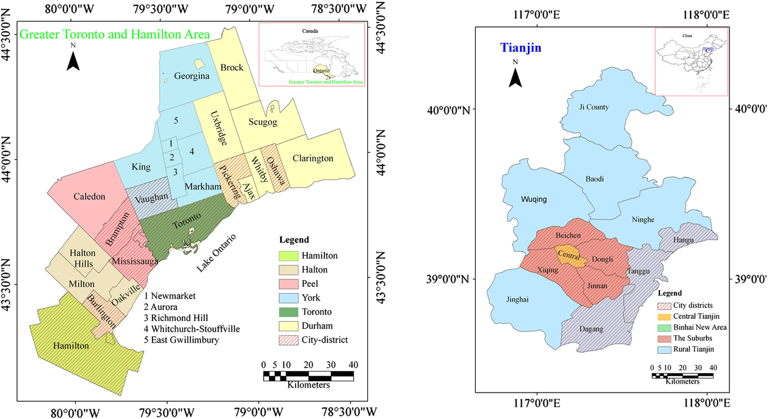
1.IntroductionNowadays, cities across the world are spreading into their surrounding landscapes, sucking food, energy, water, and resources from the natural environment and profoundly changing global ecosystems. Urban ecosystems are among the most dramatic manifestations of anthropological impacts on the environment.1,2 Recent research has also shown that urban sprawl and increased land use/land cover change in urban areas have considerable impacts on climate, hydrological, and biogeochemical cycles at various scales.3,4 Therefore, it is important to understand clearly the different urban land surface characteristics, their spatial and temporal dynamics, and the corresponding responses to regional and global environment change. The advantages of remote sensing—such as relatively low cost, large-area coverage, and repetitive observations—and also the growing interest in urban ecosystems have promoted the application of remote sensing in monitoring the urban environment. Researchers have developed a variety of approaches to distinguish surface cover types and numerous environmental variables through using remote sensing data in urban areas. Ridd2 presented a concept model to parameterize the biophysical composition of urban environments. This model, namely the vegetation–impervious surface–soil (V–I–S) model, may serve as a foundation for characterizing urban/near-urban environments and has been applied in various studies. Chen5 used Landsat TM and SPOT-P data to examine the effect of V–I–S cover types as input to hydrological models for runoff prediction for storms. Gluch et al.6 utilized advanced thermal land applications sensor data to determine urban heat island effects using V–I–S cover types. Rashed et al.7 employed four spectral bands of Indian IRS-1C imagery to study the anatomy of Greater Cairo in terms of end-member fractions (vegetation, impervious surface, soil, and shade) through linear spectral mixture analysis. Artificial neural network algorithms,8–10 such as the multilayer perception feed-forward network and the back-propagation network, were applied for estimating end-member fractions within each pixel. Based on the V–I–S fractions, the classification and regression tree (CART) algorithm has also been widely used to obtain the impervious surface end-members.11–13 More recently, some researchers have attempted a modern machine learning method—the support vector machine (SVM)—to map urban characteristics.14–17 Meanwhile, studies of quantitative landscape ecology have developed landscape spatial metrics or indices to quantify the spatial contiguity, shape, and patch distribution of classified data. A major problem is that, at the moment, it is difficult to extract accurately urban components based on remotely sensed data. Each image classifier has its own advantages and disadvantages. It is difficult to get a higher accuracy by relying on one classifier. Combining the strengths of several different methods—particularly through the synthesis of an advanced classifier and by using knowledge obtained from auxiliary data or empirical models—would contribute to producing a higher accuracy. In this paper, a machine learning methodology of global optimization—the SVM algorithm—was chosen as the classifier because of its improved performance compared to other approaches. This improved performance has been demonstrated in previous studies.15–17 In addition, two kinds of knowledge were used to help to extract urban components: geospatial auxiliary data, such as urban vector data, and spectral index models, such as the modified normalized difference water index (MNDWI)18 and normalized difference bareness index (NDBaI).19 Although the V–I–S segmentation method of land cover is superior to models or classifications of land use for energy and moisture flux analysis of ecosystems,20 there is still some spectral confusion because the same object can have different spectra or different objects can have the same spectrum. In this paper, four end-members including a high-albedo object, a low-albedo object, and easily distinguishable vegetation and soil were selected for the classification and fraction computation. After this had been done, empirical models and geospatial data were used to map this to V–I–S components. Remotely sensed information has been widely applied in urban environment studies. Multitemporal remote sensing data have been used to map urban areas and reveal urban spatial and temporal changes.20–32 Research20,23–26 demonstrates that the spatial metrics can be useful tools for monitoring a particular urban landscape by providing various measures of patch shapes and patterns. Most studies focus on case studies in developing countries21–23,28,29 or in developed countries.24,30 Moreover, comparison analyses between different countries are mostly based on coarse resolution imagery.27,31 Due to difficulties in data acquisition and data processing,6 not much research has been conducted into comparison analysis at medium resolutions. In 2011, the Comparative Study on Global Environmental Change Using Remote Sensing Technology project started. This program selects areas from China, Canada, Brazil, and Australia that are sensitive to global environmental change as test sites. Comparative studies of typical global change phenomena are performed between the northern and southern hemispheres, and also between the eastern and western hemispheres so as to develop the methodology of global environmental change remote sensing and to provide scientific data and decision support to deal with global environmental change. As a preliminary study of this project, we selected two urban areas, one in Canada and one in China, to explore the differences in urban development and the ecological implications of these differences. 2.Study Area and Datasets2.1.Study AreaThe Greater Toronto and Hamilton Area (GTHA) is located at the western end of Lake Ontario in Southern Ontario, Canada [Fig. 1(a)]. Extending from 43°17′ N to 44° 2′ N and 78°6′ W to 80°5′ W, it is the largest metropolitan area in Canada and is ranked in the top 50 most densely populated areas in the world.33 The GTHA covers the city of Toronto as well as the surrounding regional municipalities of Durham, Halton, Peel, York, and Hamilton. The city of Tianjin is located between 38.57°N and 40.25°N and between 116.72°E and 118.32°E, covering [Fig. 1(b)]. Tianjin is one of the four directly governed municipalities of China and comprises the fifth largest area of urban land in China. In terms of urban population, Tianjin is the sixth largest city in China. Since 1980, the urban population of Tianjin has grown by 50% and has now reached 10.29 million.34 2.2.Datasets and PreprocessingOwing to their unique features of a long-time span, low cost, and relatively high temporal and spatial resolution, Landsat datasets were selected as our primary datasets in this study. The Landsat ETM+ and TM data were acquired from the global land cover facility at the University of Maryland ( ftp://ftp.glcf.umd.edu/glcf/Landsat/), the U.S. Geological Survey website ( http://eros.usgs.gov), and the remote sensing data sharing platform at the Center for Earth Observation and Digital Earth, Chinese Academy of Sciences ( http://ids.ceode.ac.cn/). Four Landsat scenes (path/row of 18/29, 18/30, 17/29, and 17/30) were downloaded to cover the GTHA, while two scenes were downloaded (122/32 and 122/33) for Tianjin. Three stages of Landsat imagery from 1985 to 2005 were used to investigate the spatiotemporal dynamics of both study sites. To reduce classification uncertainty, only images that had limited cloud cover and that fell in the period of August to September (except for one 1987 scene of Tianjin) were selected. Detail descriptions of the datasets used are shown in Table 1. For the GTHA, three land use and land cover (LULC) maps (for 1985, 2001, and 2005) were provided by the Canadian Urban Land Use Survey. All Landsat scenes were processed to level 1T using the Universal Transverse Mercator map projection (UTM, Zone 17N for GTHA, UTM, Zone 50N for Tianjin), WGS84 geodetic datum, and north-up image orientation. All images and LULC maps were georegistered with RMS errors of . The LULC data were resampled to 10 m and the Landsat data were resampled to 30 m. Table 1Characteristics of satellite data used for the study area.
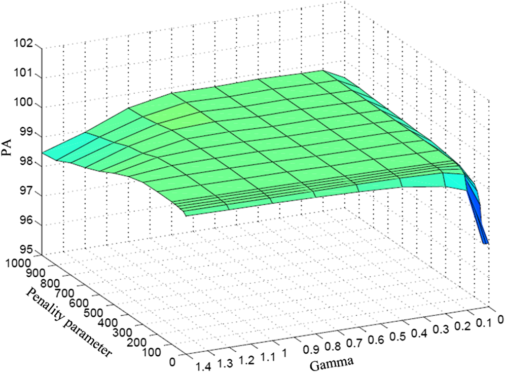
3.MethodologyIn this study, a machine learning methodology of global optimization, the SVM algorithm, was chosen as the classifier because of its improved performance, as demonstrated in previous studies, compared with other approaches.15,17 Moreover, two kinds of information were used to help to extract urban components: geospatial auxiliary data, such as urban vector data, and spectral index models.18–29,35 Statistical analysis of fraction images and spatial metric analysis were then carried out in municipal districts and metropolitan areas in both study areas. The flow chart in Fig. 2 shows the processing chain used in this study. 3.1.Support Vector MachineThe SVM originates from a nonparametric machine learning methodology that follows basic ideas of supervised classification to map data into a high-dimensional space in order to identify the hyperplane of each class.36–38 Due to its advanced generalization ability in targeting classification rules, it facilitates comparatively accurate computation and can carry out image classification processing quickly.39 In this paper, about 800 samples for each stage image were manually selected for each end-member and were used for training. These included high-albedo objects, low-albedo objects, vegetation, and soil from the original images. Meanwhile, another 800 samples were selected and used for classification evaluation. The samples were selected from the most extreme areas of the feature space with the help of Envi4.7 software models (i.e., minimum noise fraction, pixel purity index, and n-dimensional visualization) and also using LULC category information. More particularly, the vegetation samples were taken from the areas of dense vegetation cover, the impervious ones from commercial/industrial areas or major road arteries, the soil from fallow agricultural land, and the water from areas of clear, deep water. SVM uses training data to generate a model for estimating the targeted values. Training the SVM with a radial basis function requires two parameters: the penalty parameter controls the trade-off between maximizing the margin and minimizing the training error, while the gamma parameter describes the kernel width. In this study, the SVM library LIBSVM developed by Chang and Lin40 is employed. The influence of both parameters on the producer’s accuracy (PA) is analyzed in the process. In Fig. 3, the classification accuracy improves sharply at a gamma parameter of 0.1 and changes slightly in the range [0.1, 0.6]. The SVM performs better with a penalty parameter in the range [100, 300] and its accuracy decreases at larger values. To achieve a better accuracy and a faster processing time, in this study, the gamma parameter and penalty parameter were set to 0.143 and 100, respectively. 3.2.V–I–S and Knowledge-Based Mapping ModelsThe V–I–S model [Eq. (1)] is a conceptual framework that groups the great variety of urban land covers into three general categories—vegetation, impervious surface, and soil—plus water.1 where , , , , and are the reflectance for land type, impervious surface, vegetation, soil, and water, respectively, for band ; , , , and are the corresponding fractions of associated components; and is the residual error.Previous studies35,41 demonstrated that impervious surfaces were located on or near the line connecting the low-albedo and high-albedo end-members in the feature space. Therefore, the percentage covered by impervious surfaces can be estimated as a linear combination of low-albedo and high-albedo surfaces. Then, Eq. (1) can be described as where ,, , , and are the reflectance for land type, low-albedo, high-albedo surface, vegetation, and soil, respectively for band ; , , , and are the corresponding fractions of associated components; and is the residual error.Equation (2) shows that spectral reflectance of an urban surface is composed of four end-members (high-albedo objects, low-albedo objects, vegetation, and soil). The mapping model between V–I–S and the end-members was established based on Eqs. (1) and (2) and on knowledge-based empirical values of the indexes shown in Fig. 2. Generally, low-albedo materials comprise water, dark impervious surfaces (i.e., asphalt road), and shadow. Water could be easily extracted according to the low-albedo classification result and the empirical value of MNDWI () derived using Eq. (3).18 Other information such as geospatial vector data (for example, urban administrative boundaries and road network data) is very useful for separating different components that have similar spectra. Shadows in urban area make up only small proportions of the whole image and so can be ignored. Areas in shadow outside urban areas generally consist of the shaded slopes of hills, which can be separated into vegetation or soil by using the NDVI [Eq. (4)]—threshold for soil: ; otherwise, vegetation. High-albedo materials such as dry soil and sand tend to be confused with bright impervious surfaces. High-albedo impervious surfaces can be extracted by removing dry sands or dry soils with NDBaI [Eq. (5)] (dry soil: ). Following the steps in Fig. 2, we can get four fraction images of V–I–S and one V–I–S classification image. where , , , , and are the planetary top of the atmosphere reflectance in band 2, band 3, band 4, band 5, and band 6, respectively.3.3.Spatial and Temporal Analysis ModelsIn this study, we used two indicators or models to measure the spatial-temporal dynamics of the urban environment: rate of change of impervious surface and the aggregation index (AI). 3.3.1.Rate of change of impervious surfaceThis is calculated using Eq. (6) and compares the dynamic differences of urban impervious surfaces. where is the rate of change of impervious surface during the study period, and are impervious surface area or percentage at the end and beginning of the study period, respectively, and is the length of the study period measured in years. The results of this calculation give the annual rate of change of the impervious surface.3.3.2.Aggregation indexThe study also provided quantitative measures of urban growth pattern besides extent and change estimates in the two urban areas during the two stages. In the field of landscape ecology, a number of metrics have been developed for assessing urban dispersion. These include the landscape shape index, AI, split index, and so on. In this research, the AI [Eq. (7)] was selected to measure class aggregation or clumping, which increases as the patch type becomes more aggregated. The index is easily calculated using ArcGIS or Fragstats software. where is the number of like adjacencies between pixels of patch type based on the single-count method, is the maximum number of like adjacencies between pixels of patch type based on the single-count method, and is the proportion of landscape composed of patch type .In this study, the V–I–S outputs were aggregated into six classes according to impervious surface percent (ISP), that is, high albedo (ISP [0.8,1]), middle albedo (ISP [0.5,0.8]), low albedo (ISP [0,0.5]), vegetation, and soil. Then we explored the zonal spatial patterns of the six classes in the study area (as shown in Fig. 1) using a spatial metric analysis software (FRAGSTATS 3.3). 4.Results and Discussion4.1.SVM ClassificationFour classes—high albedo, low albedo, vegetation, and soil—were derived from Landsat images at each stage. Accuracy assessment was conducted only for the GTHA as only GTHA has matched evaluation data. For accuracy assessment, the confusion matrix approach was applied to extract four accuracy indicators: overall accuracy (OA), user’s accuracy, PA, and the overall kappa coefficient (OK). The confusion matrix is shown as Table 2. Table 2Confusion matrix of classification accuracies.
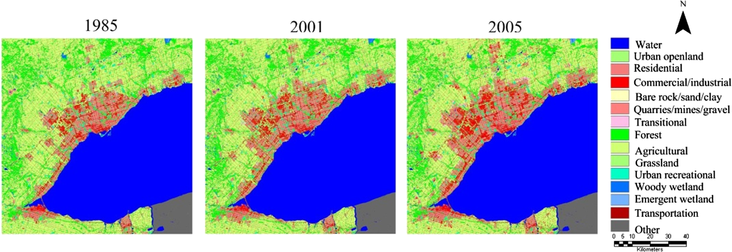
From the table, it can be seen that, in this study, this type of segmentation method produced good results with a high OA (96.69%) and high OK (95.58%). The relatively lower separability between high albedo and soil resulted in a lower PA (86.96%) compared to other end-members. 4.2.VIS Fraction ComponentsUsing the V–I–S model, four fraction images—vegetation, impervious surface, soil, and water—were developed for Tianjin [Fig. 4(a)] and the GTHA [Fig. 4(b)] in three stages. Three statistical indicators comparing the estimated V–I–S fraction and the reference data [root-mean-square error (RMSE), the mean absolute error (MAE), and the coefficient of determination ()] were used to evaluate the accuracy of the V–I–S estimation. Detailed formulae and descriptions of the assessment indicators can be found in Ref. 42. One hundred pixels were able to be selected using a random function from LULC (Fig. 5) data (only data from 1985 and 2005 were selected because of considerations of synchronicity), and based on the selected pixels, one hundred samples for statistical analysis were produced (Fig. 6). Due to the different categories in the V–I–S land surface cover and the LULC data, the classification results could not be directly compared with LULC data. For this reason, knowledge-based indexes were used to build a set of mapping rules for comparison (Table 3). In Table 3, the numbers in brackets [(1) to (9)] represent different special circumstances as determined by the LULC data, the knowledge-based indexes (NDVI and MNDWI), and empirical threshold values:18,43 case (1): , ; case (2): , ; case (3): , discard the pixel; case (4): , ; case (5): , ; case (6): , ; case (7): , ; case (8): and (2), ; case (9): and (5); case (10): for transitional urban recreational areas and other LULC, discard the sample and then reselect. The urban component fractions equal the sum of the corresponding weights of each category weight divided by the number of effective pixels (). The error statistics of the total fractional covers were calculated by comparing the V–I–S mapping model with the LULC data for the GTHA (Table 4). Fig. 6Accuracy assessment flow chart from the vegetation–impervious surface–soil (V–I–S) mapping model.  Table 3Mapping rules for mapping weights of land use and land cover (LULC) contribution to vegetation–impervious surface–soil (V–I–S) fraction (1 means 100%; 0 means 0%).
Table 4Accuracy assessment of fractional estimation results for V–I–S components.
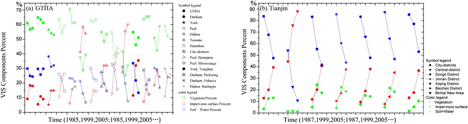
The low RMSE and MAE and high of all the fraction components also indicated the high accuracy of the approach. Among popularly used subpixel classifiers, the linar spectral mixture analysis-based method tends to overestimate the impervious surface fraction in nonurban areas and to underestimate it in urbanized areas.9 CART-based methods are more sensitive to data noise.13 Impervious surface is often confused with dry soil and water. In this case, it is difficult to accurately segment impervious surface from other objects directly. In our research, we selected the four end-members according to spectral characteristics and took advantage of the comparatively accurate and fast processing capability of the SVM algorithm and knowledge-based empirical models to obtain a higher level of accuracy. 4.3.Comparison of Spatiotemporal Patterns in GTHA and TianjinUsing the V–I–S fraction components, the spatial and temporal dynamics of each component can be easily depicted. The V–I–S components in municipal districts and metropolitan areas were extracted from the fraction images. The two graphs—one for the GTHA [Fig. 7(a)] and one for Tianjin [Fig. 7(b)]—reveal the patterns and processes of urban development in both areas. In the past 20 years, urban areas have experienced rapid growth. However, there is a great difference between the situations in the GTHA and Tianjin. For the GTHA, it mainly increased from 1985 to 1999. After 1999, only two municipal areas (Peel and Halton) and four cities (Brampton and Mississauga in Peel, Vaughan in York, and Burlington in Halton) have positive urban growth trends. In 1985, only Toronto had a high level of urbanization, while the other areas had relatively low urbanization levels. Thus, urban development in the GTHA could be regarded as having a monocentric pattern. After 1999, satellite cities or towns adjacent to Toronto, including Brampton and Mississauga in Peel and Vaughan in York, reached high levels of urbanization and became new urban centers. At the same time, other satellite cities or towns farther away from Toronto became subcenters. This could be called a multicentric urban pattern. Tianjin has experienced continuous rapid urban sprawl since 1985. Since 1999, the rate of urban sprawl has accelerated at the cost of soil and vegetation loss. In 1985, only the central district had a high level of urbanization, but in recent decades, the coastal area has developed into a new center (Binhai New Area). In the ternary diagram (Fig. 8) of the urban environment, all sites in the GTHA are near to the vegetation and impervious surface axes, while the ones in Tianjin are near to the soil (plus water) and impervious axes, which demonstrates the great differences between the two areas. In the 1980s, soil characteristics are clear for Tianjin due to the image acquisition date (May); impervious surface fractions at most sites in the GTHA are higher than in Tianjin in the 1980s and in 1999 but are lower in 2005. In addition, the impervious surface fraction for Tianjin is increasing at an accelerating rate all the time, while for the GTHA a point of inflexion has been passed. Finally, the GTHA has a high level of urban greenery, while in Tianjin it is very low. Fig. 8A dynamic ternary V–I–S diagram for municipal districts and metropolitan areas in the GTHA and Tianjin areas.  Figure 9 shows the annual rate of change in the impervious surface area for the GTHA and Tianjin. Figure 9(a) indicates that from 1985 to 1999, all sites in the GTHA had positive change rates, whereas from 1999 to 2005, the rates of change at some sites had turned negative. It can also be seen that in the first stage, York municipality and its city Vaughan had a high rate of change due to its proximity to Toronto; in the second stage, the rate of change at all sites was far slower than in the first stage. From Fig. 9(b), it can be seen that in the first stage, the rate of change was , whereas in the second stage, it had reached 25% in the Beichen district. Figure 10 illustrates the spatiotemporal dynamics of the urban growth patterns of the study areas. From Fig. 10(a), it can be seen that all districts in the GTHA became more disaggregated from 1985 to 1999 and more aggregated from 1999 to 2005. For Tianjin [Fig. 10(b)], it can be seen that more patches became aggregated in the first stage and became more decentralized in urban areas in the second stage, except for central Tianjin. 4.4.DiscussionIn this study, we used the MNDWI to remove the water from the low-albedo fraction image and used the NDBaI to eliminate dry soils from the high-albedo fraction image. The evaluation of the accuracy showed that the accuracy was high. However, we could not remove the shade from urban areas in the low-albedo fraction image, although this could correspond to impervious surface. Also, the NDBaI index could only eliminate very dry soils (primary barren soil). In the evaluation process, samples containing transitional and urban recreational areas were discarded. In fact, these areas could contain multiple categories. Therefore, we need to evaluate the validity of this method in future work, focusing on transitional urban areas. In addition, this assessment was carried out for the GTHA only due to the lack of synchronous high-resolution images for Tianjin. The spatiotemporal dynamics of the GTHA and Tianjin revealed that there were great differences between the two urban areas. This could be related to factors such as population and policy. According to census data, the proportion of the population classified as urban in Tianjin was 53.70, 57.29, and 75.11% in 1985, 1999, and 2005, respectively. In the GTHA, it exceeded 82% in 1985. Figure 11(a) illustrates population and population density in Tianjin, the GTHA, and their central cities (central Tianjin and Toronto). The most surprising feature of this graph is that the population density of central Tianjin far exceeds that of the other areas, although there is no obvious population density difference between Tianjin and the GTHA and other pairs of population and population density curves (GTHA and Tianjin; Toronto and central Tianjin) are almost parallel. The large increase in the urban population percentage in Tianjin and the high population density in central Tianjin may partly account for the rapid increase in impervious surfaces. However, population and population density increases in the GTHA and Toronto did not bring about a corresponding appreciable increase in impervious surfaces from 1999 to 2005, which implies that another factor played an important role in the urban development. Since the 1990s, experts in urban studies and environmentalists in Canada have raised concerns about the region’s rapid, low-density pattern of land development, calling for better management of future land-use decisions. The provincial government has also introduced related legislation, such as the “Places to Grow Act 2005.” In contrast, China experienced a real estate bubble in the 1990s, which resulted in a disorganized expansion of developed land. These different policy principles are another factor impacting on the dynamics of the urban ecological environment. 5.ConclusionsThis study explores the application of the V–I–S method in large-area urban agglomeration mapping and ecological environment analysis. First, four end-members (high-albedo surface, low-albedo surface, vegetation, and soil) were selected for classification using the SVM algorithm. The accuracy of the classification results reached 96.69%. Next, to map the SVM results to V–I–S component fractions, a knowledge-based method was applied to the results to establish a mapping model—the RMSE ranged from 3.12 to 6.43% and ranged from 0.94 to 0.99. Finally, a spatiotemporal analysis was conducted for municipal and metropolitan areas in Tianjin, China, and the GTHA, Canada. We found that both urban areas experienced rapid growth in the period from 1985 to 2005. For the GTHA, urban sprawl mainly occurred from 1985 to 1999. Urban development patterns underwent a change from monocentric (based on Toronto) to multicentric (based on Toronto, Brampton, and Vaughan). For Tianjin, all districts underwent rapid urban expansion, with the rate accelerating after 1999. The aggregation index results reveal that the GTHA and its municipal areas became more disaggregated from 1985 to 1999 and then more aggregated from 1999 to 2005, which implies that the Canada government’s initiatives achieved their intended result of compact growth. Most urban sites in Tianjin showed the opposite trend. The results reveal different patterns of sprawl in the GTHA and Tianjin, which may reflect the demographic and economic influences on urban environments across the globe. AcknowledgmentsThis research was sponsored by Major International Cooperation and Exchange Project of National Natural Science Foundation of China (Grant No. 41120114001) and was also supported by 973 Program “Earth Observation for Sensitive Factors of Global Change: Mechanisms and Methodologies” (No. 2009CB723906) and the National Natural Science Foundation of China “Study of Characteristics of the Environmental Field before the Strong Convective Cloud Initiated Using Geostational Meteorological Satellite Data” (No. 41005026). The authors would like to thank the U.S. Geological Survey for providing free and high-quality Landsat images and the Canadian Urban Land Use Survey for providing the land use and land cover data of the Greater Toronto and Hamilton Area. The authors also thank the anonymous reviewers and the editor for their constructive comments and suggestions. ReferencesG. HeikenR. FakundinyJ. Sutter, Earth Science in the City: A Reader, 7
–20 AGU, Washington, DC
(2003). Google Scholar
M. Ridd,
“Exploring a V-I-S (vegetation-impervious surface-soil) model for urban ecosystem analysis through remote sensing: comparative anatomy for cities,”
Int. J. Remote Sens., 16
(12), 2165
–2185
(1995). http://dx.doi.org/10.1080/01431169508954549 IJSEDK 0143-1161 Google Scholar
N. B. GrimmH. F. StanleyN. E. Golubiewski,
“Global change and the ecology of cities,”
Science, 319
(5864), 756
–760
(2008). http://dx.doi.org/10.1126/science.1150195 SCIEAS 0036-8075 Google Scholar
S. T. PickettM. L. CadenassoJ. M. Grove,
“Urban ecological systems: linking terrestrial ecological, physical, and socioeconomic components of metropolitan areas,”
Annu. Rev. Ecol. Syst., 32
(1), 127
–157
(2001). http://dx.doi.org/10.1146/annurev.ecolsys.32.081501.114012 ARECBC 0066-4162 Google Scholar
J. Chen,
“Satellite image processing for urban land cover composition analysis and runoff estimation,”
University of Utah,
(1996). Google Scholar
R. GluchD. QuattrochiJ. C. Luvall,
“A multi-scale approach to urban thermal analysis,”
Remote Sens. Environ., 104
(2), 123
–132
(2006). http://dx.doi.org/10.1016/j.rse.2006.01.025 RSEEA7 0034-4257 Google Scholar
T. Rashedet al.,
“Revealing the anatomy of cities through spectral mixture analysis of multispectral satellite imagery: a case study of the greater Cairo region, Egypt,”
Geocarto Int., 16
(4), 5
–15
(2001). http://dx.doi.org/10.1080/10106040108542210 1010-6049 Google Scholar
X. HuQ. Weng,
“Estimating impervious surfaces from medium spatial resolution imagery using the self-organizing map and multi-layer perceptron neural networks,”
Remote Sens. Environ., 113
(10), 2089
–2102
(2009). http://dx.doi.org/10.1016/j.rse.2009.05.014 RSEEA7 0034-4257 Google Scholar
Q. WengX. Hu,
“Medium spatial resolution satellite imagery for estimating and mapping urban impervious surfaces using LSMA and ANN,”
IEEE Trans. Geosci. Remote Sens., 46
(8), 2397
–2406
(2008). http://dx.doi.org/10.1109/TGRS.2008.917601 IGRSD2 0196-2892 Google Scholar
S. LeeR. G. Lathrop,
“Subpixel analysis of Landsat ETM+ using self-organizing map (SOM) neural networks for urban land cover characterization,”
IEEE Trans. Geosci. Remote Sens., 44
(6), 1642
–1654
(2006). http://dx.doi.org/10.1109/TGRS.2006.869984 IGRSD2 0196-2892 Google Scholar
L. YangC. HuangC. G. Homer,
“An approach for mapping large-area impervious surfaces: synergistic use of Landsat-7 ETM+ and high spatial resolution imagery,”
Can. J. Remote Sens., 29
(2), 230
–240
(2003). http://dx.doi.org/10.5589/m02-098 CJRSDP 0703-8992 Google Scholar
L. JiangM. LiaoH. Lin,
“Synergistic use of optical and InSAR data for urban impervious surface mapping: a case study in Hong Kong,”
Int. J. Remote Sens., 30
(11), 2781
–2796
(2009). http://dx.doi.org/10.1080/01431160802555838 IJSEDK 0143-1161 Google Scholar
J. HanM. Kamber, Data Mining Concepts and Techniques, China Machine Press, Beijing
(2007). Google Scholar
T. EschV. HimmlerG. Himmler,
“Large-area assessment of impervious surface based on integrated analysis of single-date Landsat-7 images and geospatial vector data,”
Remote Sens. Environ., 113
(8), 1678
–1690
(2009). http://dx.doi.org/10.1016/j.rse.2009.03.012 RSEEA7 0034-4257 Google Scholar
C. HuangL. S. DavisJ. R. G. Townshend,
“An assessment of support vector machines for land cover classification,”
Int. J. Remote Sens., 23
(4), 725
–749
(2002). http://dx.doi.org/10.1080/01431160110040323 IJSEDK 0143-1161 Google Scholar
G. ZhuD. Blumberg,
“Classification using ASTER data and SVM algorithms: the case study of Beer Sheva, Israel,”
Remote Sens. Environ., 80
(2), 233
–240
(2002). http://dx.doi.org/10.1016/S0034-4257(01)00305-4 RSEEA7 0034-4257 Google Scholar
Z. SunH. GuoX. Li,
“Estimating urban impervious surfaces from Landsat-5 TM imagery using multi-layer perceptron neural network and support vector machine,”
J. Appl. Remote Sens., 5
(1), 1
–17
(2011). http://dx.doi.org/10.1117/1.3539767 1931-3195 Google Scholar
H. Xu,
“A study on information extraction of water body with the modified normalized difference water index (MNDWI),”
J. Remote Sens., 9
(5), 589
–595
(2005). http://dx.doi.org/10.3321%2fj.issn%3a1007-4619.2005.05.012 Google Scholar
H. ZhaoX. Chen,
“Use of normalized differenced bareness index in quickly mapping bare areas from TM/ETM+,”
in Geoscience and Remote Sensing Symp.,
1666
–1668
(2005). Google Scholar
J. StuckensP. CoppinM. Bauer,
“Integrating contextual information with per-pixel classification for improved land cover classification,”
Remote Sens. Environ., 71
(3), 282
–296
(2000). http://dx.doi.org/10.1016/S0034-4257(99)00083-8 RSEEA7 0034-4257 Google Scholar
X. Daiet al.,
“Spatio-temporal pattern of urban land cover evolvement with urban renewal and expansion in Shanghai based on mixed-pixel classification for remote sensing imagery,”
Int. J. Remote Sens., 31
(23), 6095
–6114
(2010). http://dx.doi.org/10.1080/01431160903376407 IJSEDK 0143-1161 Google Scholar
S. HuangS. WangW. Budd,
“Sprawl in Taipei’s peri-urban zone: responses to spatial planning and implications for adapting global environmental change,”
Landsc. Urban Plan., 90
(1–2), 20
–32
(2009). http://dx.doi.org/10.1016/j.landurbplan.2008.10.010 LUPLEZ 0169-2046 Google Scholar
H. PhamY. Yamaguchi,
“Urban growth and change analysis using remote sensing and spatial metrics from 1975 to 2003 for Hanoi, Vietnam,”
Int. J. Remote Sens., 32
(7), 1901
–1915
(2011). http://dx.doi.org/10.1080/01431161003639652 IJSEDK 0143-1161 Google Scholar
A. BuyantuyevJ. WuC. Gries,
“Estimating vegetation cover in an urban environment based on Landsat ETM+ imagery: a case study in Phoenix, USA,”
Int. J. Remote Sens., 28
(2), 269
–291
(2007). http://dx.doi.org/10.1080/01431160600658149 IJSEDK 0143-1161 Google Scholar
M. HeroldH. CouclelisK. Clarke,
“The role of spatial metrics in the analysis and modeling of urban land use change,”
Comput. Environ. Urban Syst., 29
(4), 369
–399
(2005). http://dx.doi.org/10.1016/j.compenvurbsys.2003.12.001 0198-9715 Google Scholar
J. HuangX. Lu,
“A global comparative analysis of urban form: applying spatial metrics and remote sensing,”
Landsc. Urban Plan., 82
(4), 184
–197
(2007). http://dx.doi.org/10.1016/j.landurbplan.2007.02.010 LUPLEZ 0169-2046 Google Scholar
Q. ZhangK. C. Seto,
“Mapping urbanization dynamics at regional and global scales using multi-temporal DMSP/OLS nighttime light data,”
Remote Sens. Environ., 115
(9), 2320
–2329
(2011). http://dx.doi.org/10.1016/j.rse.2011.04.032 RSEEA7 0034-4257 Google Scholar
X. YuC. Ng,
“Spatial and temporal dynamics of urban dynamics of urban sprawl along two urban–rural transects: a case study of Guangzhou, China,”
Landsc. Urban Plan., 79
(1), 96
–109
(2007). http://dx.doi.org/10.1016/j.landurbplan.2006.03.008 LUPLEZ 0169-2046 Google Scholar
Y. ZhangB. Guindon,
“Analysis of urban growth pattern using remote sensing and GIS: a case study of Kolkata, India,”
Int. J. Remote Sens., 30
(18), 4733
–4746
(2009). http://dx.doi.org/10.1080/01431160802651967 IJSEDK 0143-1161 Google Scholar
L. Tole,
“Changes in the built vs. non-built environment in a rapidly urbanizing region: a case study of the Greater Toronto Area,”
Comput. Environ. Urban Syst., 32
(5), 355
–364
(2008). http://dx.doi.org/10.1016/j.compenvurbsys.2008.08.002 0198-9715 Google Scholar
A. SchneiderM. A. FriedlD. Potere,
“Mapping global urban areas using MODIS 500-m data: new methods and datasets,”
Remote Sens. Environ., 114
(8), 1733
–1746
(2010). http://dx.doi.org/10.1016/j.rse.2010.03.003 RSEEA7 0034-4257 Google Scholar
M. HashimN. M. NoorM. Marghany,
“Modeling sprawl of unauthorized development using geospatial technology: case study in Kuantan district, Malaysia,”
Int. J. Digital Earth, 4
(3), 223
–238
(2011). http://dx.doi.org/10.1080/17538947.2010.494737 1753-8947 Google Scholar
Wikipedia, “Greater Toronto Area,”
(2012) http://en.wikipedia.org/wiki/Greater_Toronto_Area#Demographics May ). 2012). Google Scholar
X. DuS. Dong, Tianjin Statistical Yearbook, China Statistics Press, Tianjin, China
(2011). Google Scholar
C. WuA. T. Murray,
“Estimating impervious surface distribution by spectral mixture analysis,”
Remote Sens. Environ., 84
(4), 493
–505
(2003). http://dx.doi.org/10.1016/S0034-4257(02)00136-0 RSEEA7 0034-4257 Google Scholar
C. J. C. Burges,
“A tutorial on support vector machines for pattern recognition,”
Data Min. Knowl. Discov., 2
(2), 121
–167
(1998). http://dx.doi.org/10.1023/A:1009715923555 1384-5810 Google Scholar
W. ChenS. HsuH. Shen,
“Application of SVM and ANN for intrusion detection,”
Comput. Oper. Res., 32
(10), 2617
–2634
(2005). http://dx.doi.org/10.1016/j.cor.2004.03.019 CMORAP 0305-0548 Google Scholar
V. N. Vapnik, The Nature of Statistical Learning Theory, Springer-Verlag, New York
(1995). Google Scholar
A. Tzotsos,
“A support vector machine approach for object based image analysis,”
(2013) http://www.isprs.org/proceedings/XXXVI/4-C42/Papers/09_Automated%20classification%20Generic%20aspects/OBIA2006_Tzotsos.pdf October ). 2013). Google Scholar
C. C. ChangC. J. Lin,
“LIBSVM: a library for support vector machines,”
(2008) http://www.csie.ntu.edu.tw/~cjlin/libsvm October ). 2008). Google Scholar
M. E. BauerB. C. LoffelholzB. Wilson, Remote Sensing of Impervious Surfaces, 59
–73 Taylor & Francis Group, Boca Raton
(2008). Google Scholar
R. A. JohnsonD. W. Wichern, Applied Multivariate Statistical Analysis, Tsinghua University Press, Beijing
(2001). Google Scholar
J. A. SobrinoJ. C. Jiménez-MuñozL. Paolini,
“Land surface temperature retrieval from LANDSAT TM 5,”
Remote Sens. Environ., 90
(4), 434
–440
(2004). http://dx.doi.org/10.1016/j.rse.2004.02.003 RSEEA7 0034-4257 Google Scholar
Biography Huadong Guo has been engaged in remote sensing research since 1977 in the field of mechanism of radar remote sensing, earth observation systems, and remote sensing applications. He was a leader of more than 10 key programs related to earth observation. He is an expert in synthetic aperture radar (SAR) and relative applications or remote sensing.  Qingni Huang received her PhD from Center for Earth Observation and Digital Earth, Chinese Academy Science in 2012 and is now working in National Satellite Meteorological Center. Her research interests include urban environment, retrieval and simulation of land surface temperature.  Xinwu Li is an associate professor in the Institute of Remote Sensing and Digital Earth, Chinese Academy of Sciences. He has published 30 papers about polarimetric and interferometric SAR remote sensing. His current research interest is global environment change especially in urban area based on remote sensing. Zhongchang Sun is an assistant professor of Institute of Remote Sensing and Digital Earth, Chinese Academy of Sciences. He has issued three science citation index papers about urban impervious based on remote sensing. Ying Zhang is a research scientist at the Canada Centre for Remote Sensing, Natural Resources Canada. She has been working on research and technical development of optical remote sensing and atmospheric physics since 1987. Her current research interests include applications of high-resolution remote sensing to urban mapping, disaster management, and sustainability issues related to natural resource development. |
||||||||||||||||||||||||||||||||||||||||||||||||||||||||||||||||||||||||||||||||||||||||||||||||||||||||||||||||||||||||||||||||||||||||||||||||||||||||||||||||||||||||||||||||||||||||||||||||||||||||||||||||