2.1.

Study Area and In Situ Measurement

The temperature data inversion in this study was a part of the hydrological modeling in ungauged regions in Central Asia. This study was carried out at the region containing runoff of the Ili River (an international river lying between China and Kazakhstan, Fig. 1) covering an area of $\mathrm{115,000}{\mathrm{km}}^2$. The outlet of the study area is the same as the outlet of the Kapchagay Reservoir. The precipitation in this area varies greatly due to the topography. Depending on the variation in topography, the precipitation in the Ili basin can reach up to $1000\mathrm{mm}/\text{year}$ in the mountains compared with $200\mathrm{mm}/\text{year}$ in the valley. The temperature also changes extensively because of the great differences in altitude.

Fig. 1

Sketch map of the study area and validation site locations.

Daily average temperature data from meteorological stations (at Yining and Zhaosu, located in the plain and mountainous areas, respectively) were collected from 2005 to 2009, corresponding to the remote sensing–based temperature simulation and hydrological modeling period. These data were collected for the derived daily average temperature validation. It is noticed that the derived daily average temperature using the Klemen method based on multisource spatial data has a height of 2 m above the surface,²⁴ while the observations from Chinese meteorological stations are recorded at 1.5 m above ground according to the “Technical regulation of meteorological observations” published by the China Meteorological Administration. The derived daily average temperature was transformed to the height of 1.5 m above ground before it was validated using observations.

A field experiment was carried out for a test site (81.10°E, 42.78°N and 2017 m altitude) near Aheyz, a southern study area (Fig. 1). The instantaneous air temperatures are recorded using the automatic meteorological station HOBO and are available at 4 min intervals from August to November in 2009 (see Table 1 for details on the instrumentation for the temperature measurements). The instant temperature recorded by HOBO was used to have the simulated instant temperature value from Klemen method tested, and the daily mean value from the HOBO records were used to validate the derived daily mean values from the Klemen method after temporal transformation and downscaled GLDAS temperature. So the measurements using HOBO were carried out 2 m above the ground to be consistent with the height described in Zakšek.²⁴

Table 1

Instrumentation (HOBO) for temperature measurements at the Aheyz.

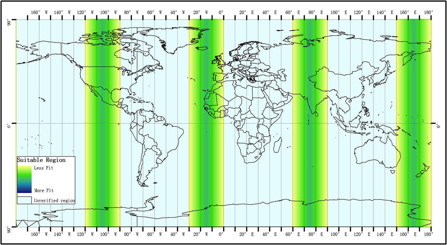
2.2.

Spatial Data

Multisource spatial data platform products were used in this study to estimate daily mean values of near surface air temperatures (${\mathrm{T}}_{2m}$), including the MODIS, GLDAS, Shuttle Radar Topography Mission (SRTM), and NCAR/NCEP products. These data products were selected for their global coverage and common use in various research fields, both of which may offer this study wider application in other regions.

Three MODIS products at 1 km spatial resolution (version 5) were used to derive the instant ${\mathrm{T}}_{2m}$: (1) 8-day albedo (MCD43B3), (2) 16-day vegetation index (MOD13A2), and (3) daily land surface temperature and emissivity (MOD11A1).

NCAR/NCEP near surface air temperature data were used in this study to transform the instant ${\mathrm{T}}_{2m}$ to a daily mean value.^26–28 This NCAR/NCEP dataset has a spatial resolution of 1.875 deg and a temporal resolution of 6 h, so there are four instant values (UTC 00:00, 06:00, 12:00, and 18:00) for each day.

GLDAS provides the near surface air temperature data with a spatial resolution of 0.25 deg and a temporal resolution of 3 h.²⁹ These data were then spatially downscaled to 1 km using the SRTM elevation data on the basis of an assumed temperature lapse rate. The downscaled results were then used to adjust the MODIS retrieval results.

All of these spatial data can be obtained through the Internet for free (MODIS http://reverb.echo.nasa.gov/reverb/; NCAR/NCEP http://www.esrl.noaa.gov; GLDAS http://mirador.gsfc.nasa.gov/; SRTM http://datamirror.csdb.cn/).

3.1.

Klemen Method–Based Daily Average Temperature Retrieval

3.1.2.

Time-scale transformation to daily average value

The temperature obtained directly from the Klemen method is the instantaneous value when the satellite (Terra) passes by, while the daily mean value is required in most hydrological models. The temporal scale of the simulated temperature must be transformed before it can be used for hydrological modeling. In this study, the time-scale transformation was based on the statistical relationship between the instant temperature and the daily mean value. Unlike in the research carried out by Colombi, few weather stations exist in the study area, so an insufficient number of observations are available to establish the relationship between instant temperature and daily mean temperature. The NCAR/NCEP reanalysis temperature data were introduced to enhance this relationship.

As described above (in Sec. 2.2), the NCAR/NCEP reanalysis temperature data provide four instant temperature values in the study area (UTC 00:00, 06:00, 12:00, and 18:00) each day. The local time in the study area is $\sim 5\mathrm{h}$ before the UTC time, which means that the UTC 06:00 is approximately 11:00 in the study area, very close to the time the satellite (Terra) passes this region (the time that Terra passes the study area varies in local time from about 10:00 a.m. to about 12:00 a.m.). If we premise two simple assumptions, the daily average temperature can be derived: (1) a strong relationship exists between the NCAR/NCEP 06:00 temperature and the daily mean NCAR/NCEP temperature and (2) the same relationship exists between the derived instantaneous Klemen ${\mathrm{T}}_{2m}$ and the simulated daily mean temperature.

Figure 2 shows 10 NCAR/NCEP pixels of the study area and the relationship between the instant temperature value (UTC 06:00) and the daily mean value (the mean of the four NCAR/NCEP instant values) that was established for each pixel [Eqs. (2) to (11)].

Eq. (2)

$$\mathrm{NCEP}42\_24:y=0.85x-1.87R^2=0.96\mathrm{RSMD}=1.43°\mathrm{C},$$

Eq. (3)

$$\mathrm{NCEP}43\_24:y=084x-1.96R^2=0.98\mathrm{RSMD}=1.59°\mathrm{C},$$

Eq. (4)

$$\mathrm{NCEP}44\_24:y=0.82x-1.81R^2=0.97\mathrm{RSMD}=1.68°\mathrm{C},$$

Eq. (5)

$$\mathrm{NCEP}45\_24:y=0.82x-1.86R^2=0.98\mathrm{RSMD}=1.49°\mathrm{C},$$

Eq. (6)

$$\mathrm{NCEP}46\_24:y=0.84x-2.83R^2=0.98\mathrm{RSMD}=1.53°\mathrm{C},$$

Eq. (7)

$$\mathrm{NCEP}42\_25:y=0.92x-5.72R^2=0.96\mathrm{RSMD}=1.57°\mathrm{C},$$

Eq. (8)

$$\mathrm{NCEP}43\_25:y=0.87x-4.11R^2=0.98\mathrm{RSMD}=2.69°\mathrm{C},$$

Eq. (9)

$$\mathrm{NCEP}44\_25:y=0.87x-4.18R^2=0.97\mathrm{RSMD}=1.95°\mathrm{C},$$

Eq. (10)

$$\mathrm{NCEP}45\_25:y=0.85x-1.92R^2=0.97\mathrm{RSMD}=1.88°\mathrm{C},$$

Eq. (11)

$$\mathrm{NCEP}46\_25:y=0.83x-1.93R^2=0.98\mathrm{RSMD}=2.10°\mathrm{C}.$$

Fig. 2

Location of the National Center for Atmospheric Research/National Centers for Environmental Prediction pixels over the study area.

Good correlation between the instant NCAR/NCEP value (UTC 06:00) and the daily mean value (obtained from NCAR/NCEP instant values) can be found from Eqs. (2) to (11), each of which stands for the linear relationship between the NCAR/NCEP 06:00 instant temperature and the daily mean NCAR/NCEP temperature within each NCAR/NCEP pixels. The $R^2$ of these statistical equations vary from 0.96 to 0.98 and most RMSE are $<2°\mathrm{C}$, proving the validity of assumption 1 in all 10 NCAR/NCEP pixels.

Though assumption 2 was not directly proven like assumption 1, it is still supported indirectly by the following analysis. The NCAR/NCEP reanalysis data were generated through data assimilation system using multisource observations with advanced quality control and monitoring components.^26–28 It is widely used in the research and climate monitoring communities. So the NCAR/NCEP air temperature values in this study were supposed to be adequate to demonstrate the comprehensive conditions within NCAR/NCEP pixels, and the temporal scale transformation equations [Eqs. (2) to (11)] from the statistical analysis of NCAR/NCEP data are reasonable and representative within NCAR/NCEP pixels. As described above, the time of the derived instantaneous ${\mathrm{T}}_{2m}$ was close to the time of NCAR/NCEP 06:00 temperature, so the temporal scale transformation equations between NCAR/NCEP 06:00 temperature and daily mean value based on assumption 1 of using reanalysis temperature data can be applied to estimate the daily mean temperature using derived instantaneous ${\mathrm{T}}_{2m}$.

In addition, the derived instantaneous ${\mathrm{T}}_{2m}$ data using Klemen method has higher spatial resolution than the NCAR/NCEP pixels, so there are many instantaneous ${\mathrm{T}}_{2m}$ pixels within an NCAR/NCEP pixel. In this study, the temporal scale transformation equation of each NCAR/NCEP pixel was applied to the smaller ${\mathrm{T}}_{2m}$ pixels within its coverage.

3.2.

New Daily Average Temperature from Downscaled GLDAS Data and Klemen Method

The GLDAS temperature data were used to improve the simulations accuracy at low temperatures from Sec. 3.1. Original GLDAS datasets provided the near surface air temperature with a high temporal resolution of 3 h and a coarse spatial resolution of 0.25 deg. Before adjusting the simulated temperature data based on the MODIS products, the GLDAS temperature data were downscaled to the resolution of the MODIS grid size.

The downscaling process rested on an assumption that the GLDAS temperature value of each grid represents the average condition within this grid, so the GLDAS temperature value of each grid should equal the temperature at the average elevation of the grid. On the basis of this assumption, we introduced the temperature lapse rate to quantify the extent of temperature change with elevation [Eq. (12)]. Along with the prerequisites described above, the core of this method is the introduction of a higher (compared with GLDAS) spatial resolution (1 km) digital elevation model (DEM) refining the spatial distribution of the GLDAS temperature value and proper temperature lapse rate value assignment.

The lapse rate at which air cools with elevation change varies from $\sim 0.98°\mathrm{C}$ per 100 m for dry air (i.e., the dry-air adiabatic lapse rate) to $\sim 0.40°\mathrm{C}$ per 100 m (i.e., the saturated adiabatic lapse rate).³³ In this study, the temperature lapse rate was fixed at $0.56°\mathrm{C}/100\mathrm{m}$ according to the previous research work carried out in the study area.³⁴ The downscaling of GLDAS consists of four steps: (1) the original GLDAS daily mean temperature data (the mean value of eight 3 h instant temperature values) was calculated; (2) the average elevation with the spatial resolution of $\sim 25\mathrm{km}$ matching the original GLDAS grid size was prepared; (3) the temperature at sea level with a spatial resolution of 25 km was calculated according to Eq. (12) using data from (1) and (2) and then bilaterally interpolated to 1 km; (4) the final downscaled temperature result with a spatial resolution of 1 km was calculated by data from (3) and DEM (1 km) using Eq. (12). Figure 3 gives the procedure for downscaling.

Fig. 3

Flow chart of the global land data assimilation system (GLDAS) temperature downscaling. ${\mathrm{T}}_{\text{sea}}$ and ${\mathrm{T}}_{\text{cell}}$ mean the air temperature at sea level and pixel, respectively. ${\mathrm{H}}_{\text{cell}}$ is the pixel elevation and $\delta$ means the temperature lapse rate.

Based on the two daily mean air temperature data calculated above, new combined temperature data were generated. According to our simulation results (details in Sec. 4), the daily mean values based on the Klemen method show good heterogeneity of spatial distribution of temperature and perform better over a certain threshold, with these values becoming less accurate below this threshold. The downscaled GLDAS daily mean temperature data were used to replace the values based on the Klemen method under the threshold because of their higher accuracy compared with the station observations at low temperature. However, above the threshold, the values based on the Klemen method were retained because of their ability to represent the spatial heterogeneity of temperatures affected by various underlying parameters, unlike the downscaled temperature data, which are dominated by elevation only. The flow chart of the new daily mean temperature data generation is shown in Fig. 4.

Fig. 4

The flow chart of daily average temperature estimation using the combined method.

4.1.

Klemen Method–Based Daily Average Temperature

As described above, the station observations used in this study were recorded at a height of 1.5 m, which differs from the height of simulated surface daily average air temperature. So, before the validation was carried out, the simulations were transformed to the height of 1.5 m. The temperature lapse rate in Sec. 3.2 was used for this transformation. The lapse rate at $0.56°\mathrm{C}/100\mathrm{m}$ should be appropriate and reasonable for the reason that it was from the local study in this region based on the weather stations observations.

4.1.1.

Derived instantaneous temperature

The instant air temperature was simulated and validated with the field observations. The recorded instantaneous air temperature using HOBO at Ahyz was selected according to the transit time of the Terra satellite. The simulation results and HOBO observations with comparable time were then used for the accuracy analysis. Because of the data missing from the MODIS products (no values were available in some image pixels), only part of the observations from HOBO during the observation period have matched simulated values (Fig. 5).

Fig. 5

Derived instantaneous temperature validation use HOBO observations.

The derived instantaneous temperature has a satisfactory result. The results indicate that the instantaneous air temperature based on multisource spatial data has a high correlation with the observations, and the $R^2$ can be as high as 0.73 and the RMSE between derived air temperature and observed values is 2.65°C.

4.1.2.

Daily average temperature

The derived instantaneous air temperature was transformed to a daily average value and was then validated using the observed daily average temperature from 2005 to 2009 at the Zhaosu and Yining stations; the daily mean temperature observations from HOBO equipment were also used.

Figure 6 shows that the daily average temperature after temporal transformation was less accurate compared to the instantaneous values (Fig. 5). The RMSE and $R^2$ at the Zhaosu station during the simulation period are 4.9°C and 0.91, respectively. These two indexes performed better at the Yining station where the RMSE is 4.19°C and the $R^2$ is 0.94. When validated using the observed HOBO daily average air temperature, the results based on the Klemen method have a good performance, where the $R^2$ is 0.79 and the RMSE is 2.29°C. According to Fig. 6, the derived daily average temperature was more consistent with the observations at high temperatures. The simulated daily average temperature was lower than the actual value when the temperature was low, and the difference increases as the temperature decreases. The threshold is $\sim 0°\mathrm{C}$.

Fig. 6

Derived daily average temperature validation based on Klemen’s method using observations from the Zhaosu (a) and Yining (b) stations during 2005 to 2009 and HOBO (c) from August to November in 2009.

4.2.

New Daily Average Air Temperature

Similarly, the observed daily average temperature from 2005 to 2009 at the Zhaosu and Yining stations, and the observations from HOBO were also used for downscaled GLDAS daily average temperature validation. The results are shown in Fig. 7.

Fig. 7

Validation of the GLDAS temperature downscaling data at Zhaosu (a) and Yining (b) stations during 2005 to 2009 and HOBO (c) from August to November in 2009.

As shown in Fig. 7, the downscaled GLDAS daily average temperature performed well at both weather stations. According to the regression analysis, the $R^2$ at the Zhaosu station is 0.96 and the RMSE is 2.27°C during the simulation period, while the $R^2$ and RMSE at the Yining station are 0.96 and 2.73°C, respectively. According to the validation at HOBO location, the downscaled GLDAS data have a similar accuracy as the data from the Klemen method. The $R^2$ and RMSE are 0.86 and 2.26°C, respectively.

The new daily average temperature data comprised a combination of the derived daily mean temperature on the basis of remote sensing and the downscaled GLDAS data. Through the analysis of Fig. 6, 0°C was selected as the threshold value mentioned in Sec. 3.3 to determine if the simulated daily mean temperature using the Klemen method should be replaced with the GLDAS downscaled value.

The new daily average temperature shows significant improvement at low temperatures compared with data obtained using the Klemen method (Fig. 8). During the simulation period, the $R^2$ between the combined daily average temperature and observations from the Zhaosu station was 0.90, and this value was 0.94 at the Yining station. The RMSE at the Zhaosu station is 3.38°C, while the RMSE is 3.13°C at the Yining station.

Fig. 8

Validation of the new derived daily average temperature using observations from the Zhaosu (a) and Yining (b) stations during 2005 and 2009.

5.1.

Klemen Method–Based Daily Average Temperature

The instantaneous temperature simulated on the basis of multisource spatial data using the Klemen method performs better than the daily average value derived by temporal transformation. Two factors can possibly explain the obvious decrease in accuracy: temporal transformation and the characteristics of the Klemen method.

The relationship between the instantaneous temperature at the satellite transit time and the daily mean value was assumed to be linear in this study. This simplification will certainly introduce uncertainties. The relationship established using NCAR/NCEP data stands for the comprehensive level within each NCAR/NCEP grid. Error will also be introduced when this relationship was used in pixels with higher spatial resolution. However, considering the high correlation between the temperature at the transit time and the daily average value described in Sec. 3.1.2, the high accuracy of the simulations validated using HOBO observations at both instant and daily time scale, and the obvious underestimation shown in Fig. 6 for low temperatures, the temporal transformation should not be primarily responsible for the decrease in accuracy in the daily average temperature simulation.

Equation (1) in Sec. 3.1.1 indicates that many parameters were included in the Klemen method to depict the influence of various factors, such as radiation, season, vegetation, and topography. The air temperature derived on the basis of this method shows sufficient spatial distribution details, and the spatial pattern of the air temperature depending on the underlying surface conditions is more reasonable (see Sec. 5.3). The Klemen method was proposed by Zakšek²⁴ using observations (from May to December 2005) from dozens of meteorological stations in Slovenia, Germany, and France. Due to the warm and humid climate in Europe, most of the observations from these stations in 2005 fell into the temperature span above 0°C. Thus, Eq. (1), which is based on these observations, may be innately more suitable for use at high temperatures. The simulated instantaneous air temperature and daily average air temperature validated using HOBO observations [Figs. 5 and 6(c)] have high accuracy and may profit from the field observation time between August and September, when the temperature is high. The climate conditions in the study area are different from where Eq. (1) was established; the temperature span is wider and more low temperatures ($<0°\mathrm{C}$) appear, which may make the regional LST and NDVI in the study area no longer fit the relationship calibrated in Europe at low temperatures.

In this study, no further atmospheric correction was applied to the LST data from MODIS products. The atmospheric effects such as air moisture were partly removed or corrected when the LST was generated using the generalized split-window method; the accuracy of MODIS LST is $\sim \pm 1\mathrm{K}$. The air moisture, which will become lower and drier at low temperatures, will certainly influence the simulation accuracy, but it should not mainly account for the low simulation accuracy of this method (the overall RMSE of daily average simulation is $>4\mathrm{K}$, Fig. 6) at low temperatures.

In addition, in this study, the transformation equations obtained at coarse spatial resolution based on NCAR/NCEP data were applied to the smaller ${\mathrm{T}}_{2m}$ pixels within each NCAR/NCEP pixel with MODIS grid size. Uncertainties will be introduced in this procedure because the statistical relationship between instant air temperature and the daily average values vary when the spatial resolutions change. This method was carried out for its simplicity and feasibility in the data sparse area where the transformation equations with high spatial resolution are difficult to establish and the computational burden will be heavy. In further study, more spatial resolution independent transformation equations are needed.

5.2.

Downscaled GLDAS Daily Average Temperature Data

The downscaled GLDAS daily average temperature performed better at two validated weather stations than the data based on the Klemen method [Figs. 7(a) and 7(b)]. The RMSE between the downscaled data and the observation is within 3 K, while the RMSE is $>4\mathrm{K}$ in Figs. 6(a) and 6(b). Though the downscaled data have better accuracy at the stations, this improved accuracy did not equate to higher data quality. The downscaling process was based on the temperature lapse rate and the assumption of a relationship between the air temperature and the elevation (see Sec. 3.2). During this process, no factors other than elevation in this area were taken into account to downscale the GLDAS air temperature data. Without considering the underlying surface complexity, the downscaled GLDAS temperature data may face challenges where the underlying surface conditions (water surface, dense vegetation, aspect, and so on) have significant influences. The comparison between Figs. 6(c) and 7(c) shows that the data from downscaled GLDAS and the Klemen method have similar accuracy or the data from the Klemen method perform a little better at high temperatures using HOBO observations during the observation period. It is reasonable to believe that the downscaled daily average air temperature may not be more accurate than the data from the Klemen method for other locations (such as the valley in Fig. 9) when the temperature is high.

Fig. 9

Comparison of the results from three daily average temperature retrieval methods (take the 275th day in 2005, for example). (a) Results from the Klemen method after temporal transformation. (b) Downscaled GLDAS data. (c) Integrated daily average temperature data.

The reasonable regional spatial distribution and interrelation of parameters are important in the hydrological or ecological applications. The spatial pattern of the downscaled air temperature data was determined only by the elevation, following the variation of DEM. Due to more physically based parameters being introduced into the simulation using the Klemen method, the derived daily average temperature has a better spatial pattern and a better depiction of the distribution, especially at high temperatures.

In addition, though the temperature lapse rate used in the spatial downscaling of GLDAS data and in the process of translating the derived daily air temperature data to the height of 1.5 m above the ground was based on previous study in this area using meteorological observations, problems still exist. The temperature lapse rate in this study was fixed to the constant for the whole study area while values with spatial variation are more reasonable, though it is difficult to obtain the spatial distribution of lapse rate in the data sparse region. The temperature lapse rate is more suitable to demonstrate the variation of temperature with elevation in large scale, so it may be coarse to use the temperature lapse rate for the temperature transformation with only 0.5 m height differences. A more accurate algorithm should be discussed in further study to eliminate the height differences in the simulated daily average temperature and observations.

5.3.

New Daily Average Temperature Data

The new data were generated from the combination of the two daily average air temperatures discussed previously. Due to the discussion in Sec. 5.2, the daily average temperature based on the Klemen method was adopted at high temperatures ($>0°\mathrm{C}$) to keep its reasonable spatial pattern and was replaced by the downscaled GLDAS temperature data (see Sec. 3.2) to increase the accuracy at low temperatures ($<0°\mathrm{C}$).

At high temperatures, more details about the air temperature distribution are shown in Figs. 9(a) and 9(c), reflecting the influence of various underlying surface conditions. A large reservoir named Kapchagay exists in the study area downstream of the Ili River. The water surface evaporation cools the air above the reservoir leading to temperatures (dark gray area under the red rectangle) lower than the surrounding temperatures. A large area of the Gobi Desert lies within the study area (the bright parts), where the temperature is obviously higher. Most of the light gray areas in Figs. 9(a) and 9(c) cover well-developed vegetation. Many of these spatial pattern details cannot be seen in the downscaled air temperature distribution [Fig. 9(b)].

At the low temperatures [the black areas in Fig. 9(a)], most of which appear on the top of the mountain, the data from the Klemen method become less accurate. A useful spatial texture of the air temperature can no longer be observed, and the accuracy of the simulated temperatures obviously decreases. The downscaled GLDAS air temperature data with the DEM texture were used.

In this study, the derived daily average air temperature based on the Klemen method was simply replaced with the downscaled GLDAS data to achieve overall simulation accuracy. In the future, weights may be introduced to integrate these two temperature data. Different weight values according to certain rules will be assigned to the Klemen method data and the downscaled GLDAS data to reflect the contributions from each, instead of simply replacing one with another. In order to achieve better overall simulation accuracy, the coefficients used in the Klemen method can also be recalibrated in a wider temperature span to make it more suitable in different regions.

The temporal scale transformation equations used in this study were based on the NCAR/NCEP reanalysis temperature data (details in Sec. 3.1.2). NCAR/NCEP provides four instant values (UTC 00:00, 06:00, 12:00, and 18:00) each day. If the Terra passing time in certain regions is close to any of the four times, the temporal scale transformation equations and the daily average air temperature can be made in the same way. In this study, the time that satellite passes the study area varies from about local 10:00 a.m. to about local 12:00 a.m., is about an hour before or after the UTC 06:00 (local time 11:00 a.m.). So that the local satellite passing time is close to any of the four NCAR/NCEP time means the difference between them is $<1\mathrm{h}$. Figure 10 shows the regions around the world where the daily average air temperature deriving method in this study can be used.

Fig. 10

Regions (four gradient color regions) fit for the daily average air temperature retrieving method in this study. The applicability of this method in other regions (with background blue) is unverified.