1.

Introduction

Currently, remote-sensing techniques construct observation systems from the ground upward for the applications of global detection and monitoring. With multilevel, multiangle, multifield spatial data, remote sensing is of great importance for the Earth’s resources and for environmental research.¹ Since the 1960s, thermal infrared imaging, airborne synthetic aperture radar, multipolar, surface-penetrating radar, and high-resolution, space-borne synthetic aperture radar technologies have become more sophisticated. The spectral regions covered by remote sensing extend from the earliest visible spectrum to near-infrared, shortwave infrared, thermal infrared, and microwave direction.² This spectral domain adapts to a variety of characteristic reflection peak wavelengths and the radiation spectrum distributions of different substances.

Nonetheless, even if current remote-sensing technology provides more spatial information than previous ones, remote-sensing data with discontinuous spatial and temporal resolutions remain inadequate. Some common predicaments, such as the absence of data at a desired location, at a specific time, or at a specific resolution, remain unsolved. These problems are particularly prominent in responses to natural disasters, such as earthquakes or tsunamis, which require high-resolution spatial data within 72 h for rescues; it is almost impossible to obtain them given the uncertainties of disaster sites.

Geographical data evolution is a high-precision, real-time, spatial data computational deduction to compensate for the gap in spatial and temporal resolutions in remote-sensing data. Its basic procedure starts with the static remote-sensing data of specific spatial and temporal resolutions; through the dynamic simulation of geological phenomena, real-time calculations generate new data for any required time and spatial resolution.

The dynamic simulations of geographical phenomena offer an excellent opportunity; however, they are also a critical bottleneck for geology research and study in the near future. The Earth, a complex and changing system, controls its past geographical evolution, current conditions, and future environments; it also affects human beings. Three issues are put forward in the New Research Opportunities for Earth Science released by the National Research Council in 2012;³ these include interpretation techniques for recording Earth changes and extreme event data, devices for observing Earth’s current activities, and computer technology for simulating the dynamic geographical process. This innovative research, which combines interpretation techniques, multiple time and spatial observation dates, and dynamic simulations of geographical phenomena through computer technology will profoundly affect future Earth’s science research.

However, geographical data evolution calculation faces many difficulties. The existing spatial data model cannot be applied to simulate dynamic geographical phenomena. A three-dimensional (3-D) spatial data model is the spatial information carrier and also the direct object of computer calculations. On one hand, a 3-D model must be acclimated to the expressions of the physical structure and the driving forces of geographical objects; on the other hand, it must facilitate the mapping algorithm of physical information and computer data types. However, traditional models, such as the 3-D surface data, voxel, spatial temporary, and hybrid models, need not be designed for the spatial information representation of dynamic phenomena. First, their goals are to store static spatial information from different observations such as remote sensing and ground surveys. They lack information on data-driven mechanisms and dynamic evolutions, which are crucial for computer-supported dynamic simulations of geographical phenomena. Second, the 3-D spatial data model also determines the type and efficiency of evolution calculations; for example, the classical shortest path algorithm is much more efficient in a vector data model than in a raster data model.

In this article, we have taken a stylized geographical data evolution methodology as our goal; we employ snow simulation as the application instance and analyze the whole representative procedure in order to achieve geographical data.

The subsequent parts of this article are divided into six sections: Section 1 introduces the existing 3-D geographical data models and analyzes their shortcomings. Section 2 introduces a particle system model from the 3-D visualization field and examines its potential for expressing geographic phenomena. Section 3 is a dynamic simulation of snow; it describes the construction and calculation of the 3-D particle-based data model used to express snow. Section 4 defines the interaction methods between snow phenomena and basal remote-sensing data. Section 5 discusses the key steps and critical issues in snow simulation and the remote-sensing data evolution process, and it extracts the common geographical data evolution methodology. Section 6 summarizes the research and proposes the future issues.

2.

Analysis of Existing Three-Dimensional Geographical Data Models

So far, many scholars in the geology field have researched the 3-D data model. There are three types of this model, each based on a space partition mode: the mosaic (voxel) data, vector-based (surface) data, and hybrid models.

The mosaic data model divides 3-D space into a series of connected but not overlapping geometric elements with simple structures and permits the easy analysis of spatial characteristics. However, its geometric precision in expressing spatial position is low and not suitable for conveying and analyzing the spatial relationship between entities. At the same time, the amount of data is large, and the processing speed is slow. The common methods of mosaic-based data models are cell decomposition, spatial occupancy enumeration, the tetrahedral network, K-simplex partition, and constructive solid geometry (CSG).

The voxel model can be seen as the 3-D extension of the two-dimensional (2-D) raster data model.⁴ It uses a 3-D unit with a certain volume to pack and construct the 3-D entity model. Unlike the surface model, it is a “true” 3-D data model with its own shortcomings. It is convenient to update inner structure, but difficult to model complex entities, nor does it have the ability to maintain the topological relationship. Obvious shortcomings exist in the graphic display (depth test and observing cone cutting), spatial analysis, and spatial index, so it is difficult applying the model widely in dynamic simulation modeling of geographical phenomena (Table 1).

Table 1

Three main kinds of geographical 3-D data models.

Vector-based (surface) data model	Mosaic-based (voxel) data model		Hybrid model
3-D triangulated irregular network (TIN)	Regular voxel	Irregular voxel	TIN + voxel; Grid + TIN;Grid + vector + TIN; TIN + temporal information; ….

The vector-based data model discretely divides the 3-D space into a geometric body, whose basic definition is its boundary. It is the application of the 2-D vector model (dot-line-surface) in 3-D space. This model abstracts an entity as four basic elements in 3-D space—dot, line, surface, and body; these are later used to construct more complex objects. The vector models most often employed are B-representation (B-Rep), 3-D data, vector 3-D data, and space-partition-based spatial data models.

There are noticeable advantages of the surface model, both in its geometric descriptions and model maintenance of space objects.⁵ For example, it is easy to realize multiresolution visualization and model updating and it is suitable for network analysis and calculations, such as linear distance analysis and moving animation, as well as for space indexes and calculations, such as width traversal.⁶ However, it is not really 3-D; it cannot describe the relationship between the partition and topology of 3-D space, nor can it conduct an analysis and calculation of 3-D space in the real sense, since the mesh units in the surface model, which is only a slice of the spatial entity perpendicular to the normal direction, do not take up space in the normal direction.

Until now, 3-D data models have had their own advantages and shortcomings. On one hand, the surface-based data model represented by B-REP can express all the spatial information of geographical entity shapes and information about their topologies and sequences, but it is difficult for the model to convey its own inner spatial information or that of its constituents. It is likewise hard for the model to express complex space bodies.⁷ On the other hand, the volume-element-based data model represented by CSG can express the spatial information of geographical entity constituents and acquire geometric measuring information through Boolean operations, but it is difficult for the model to depict topology, sequence information, or irregular space.

Some spatial-temporal hybrid data models, such as the ground-state correction model, define a time dimension, and the time value is simply connected to the spatial data. The time expression in the data models is discrete; time information is more like attribute tags rather than continuously dynamic data objects. Overall, these 3-D data models are still static spatial data models, which cannot express dynamic phenomena. It is necessary to study 3-D data models more deeply.

3.

Introduction of the Particle System (3-D Particle Model)

Along with the geographical field, the data model problem also appears in 3-D visualization. There are a large number of special objects with irregular boundaries such as fountains, rain, and snow, whose movements cannot be represented by a unique equation. To solve this problem, Reeves⁸ has proposed a method to simulate irregular objects, the particle system method, in which many small particles with simple shapes and life are used to stand for irregular and obscure objects and phenomena.

A transmitter in the particle system controls the small particles’ positions and movements in 3-D space.⁸ The parameters of the particle behavior include the formation speed of particles (the number of particles produced in a unit of time), the initial velocity vector of particles (the direction of movement at certain time), particle life cycles (how long they exist), particle colors, particle life cycle changes, as well as other parameters. Instead of absolute values, the probability values of all or most of these parameters are used to express the obscure natural phenomena.

There are two different stages in the renewal of a typical particle system: the motion simulation stage and the rendering stage.⁸ During the motion simulation stage, the number of new particles can be worked out according to their formation speeds and renewal intervals, and every particle is produced in specific 3-D space according to the transmitter’s position and the preset producing area. The speed, color, and life cycle of each particle can be initialized according to the transmitter’s parameters. Next, each particle’s life time must be checked to guarantee that it exists no longer than its life cycle; otherwise, it would change in its position and features according to the physical simulation.

Normally, the geometric shape of each particle is expressed by a quadrangle or a triangle mapped by texture (sprites), which is not necessary. When the resolution is low or the treatment ability is limited, the particles should be rendered into pixels whenever possible⁹ (Fig. 1).

Fig. 1

Flames of particle system simulation.

Although the particle system can vividly express some natural phenomena, it is still a complement to the current surface model. The particle system cannot express objects with solid boundaries, reflect real-physical movement, or support a highly accurate dynamic simulation of geographical phenomena without a well-designed driving algorithm.

As a revision of the particle system and the 3-D particle data model, the procedure for building a particle data model for geographical phenomena simulation is comprised of four steps (Fig. 2):

Fig. 2

Procedure for building a simulation model of geographical phenomena based on particles.

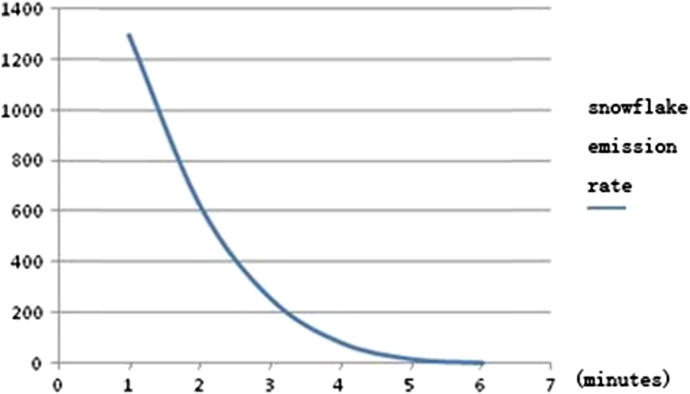
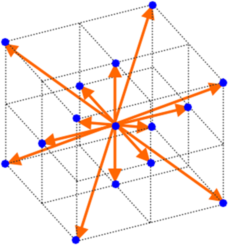
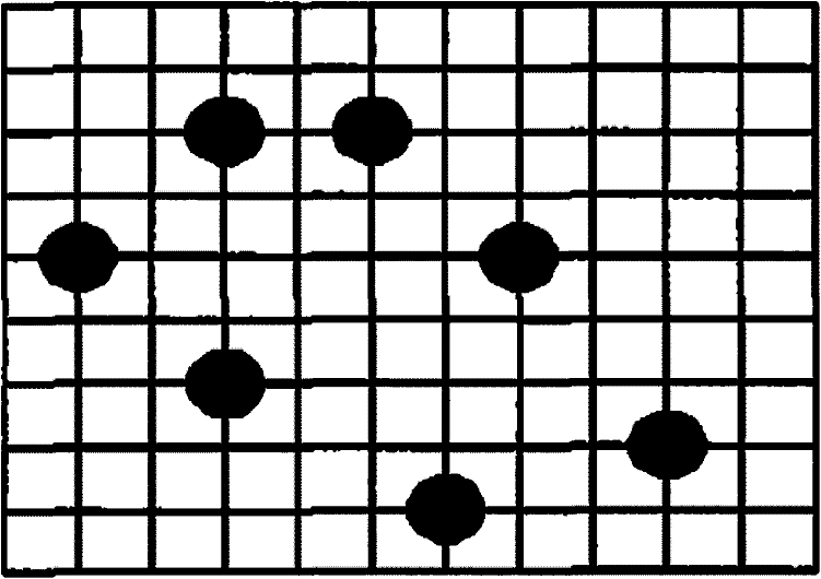
4.

Dynamic Simulation of Snow

Studying the dynamic simulation of snow is not only important for disaster prevention, but it is also an essential component of geological environment dynamic simulations. Additionally, snow is widely distributed all over the world (except for a few tropical and subtropical areas), making it an important phenomenon of the geological environment and a critical part of the hydrological cycle. This means that real-time prediction research on snow has a significant impact on the systematical observation and prediction of global climatic change and the extraction and analysis of sensitive factors. Some studies on snow phenomenon have been conducted such as avalanche risk analysis and snow melt water calculations.¹⁰ With basic observational data, such as temperature, wind speed, wind direction, and topography, the dynamic simulation of snow predicts spatial distributions during a given time and in a designated region including the real-time simulations of snowfall and snow deposit calculations.

In 1995, Masselot and Chopard analyzed the fluttering of snowflakes in wind; however, they only focused on a 2-D situation.¹¹ In 2004, Langer et al. attempted to simulate a snow scene with a graphic method to solve the speed problem that results from a number of particles;¹² therefore, they employed a series of 2-D images to simulate the snow scene with 3-D snow particles. However, they still adopted image-filtering methods to simulate the statistical properties of snowfall spatial distributions, ignoring the influence of wind and airflow, both of which caused a low-quality simulation. In 2006, Saltvik et al.¹³ also conducted experiments on simulations of snow and snow scenes with the parallel method. This method supported much more snow particles in the scene than before, but it had an obvious defect in the dynamic deposit simulation of the snow, in which it did not adopt the particle system model and did not include any interaction between wind and snow. In China, Wang et al.,¹⁴ in 2003, simulated real-time rain and snow based on a particle system, but the simulation was relatively simple and neglected dynamics equations and visualization features. In 2005, Kowira conducted further research, which generated rain and snow particles with the particle system and OpenGL texture fusion technology, clearly demonstrating visualization features but still ignoring dynamics equations. ¹⁵ Chen et al. adopted the fractional brownian motion statistical feature to show the density of snowfall; they produced an excellent result in the simulation of snow spatial distribution; unfortunately, they failed to conduct further research on snow motion simulation.¹⁶

The dynamic simulation of snow is a systematic project. Past studies have emphasized the external features, such as spatial distribution, but ignored the packaging and expression of the physical properties of snow particle units. As a result, they have achieved some visualization features or the simulation of some phases of snow motion, but could not express the entire snow process from its formation to its collection, and could not achieve the dynamic simulation of snow and real-time predictions. Additionally, we should notice that a particle system model could be used to simulate geographic entities with rich details in multiscale, discrete spatial distributions and relatively difficult shapes and can be adopted and further improved by the dynamic simulation of snow research.

In the modeling process based on the particle system mentioned above, the procedure of studies on the dynamic simulation of snow is as follows: First, they extract the minimum calibration scale of snow. Snow, as a sort of a geographic phenomenon, has a self-evident minimum unit, the snowflake. Obviously, different sized snow scenes consist of integer multiples of single snowflakes, which are closely connected to the features of diverse spatial snow motion and the minimum indispensable unit of snow, while also possessing independent motion features and uniformed physical properties.

In accordance with the observational and statistical data,¹³ the diameter range of a snowflake is between 0.05 and 4.6 mm, indicating the difficulty of crystalline lens absorption of water vapor in the atmosphere. This follows the rule that the higher the temperature, the greater the water saturation, thus leading to larger snowflakes. For example, when water saturation is 80% and the temperature is $-36°\mathrm{C}$, the average diameter of a snowflake crystalline lens is 0.1 mm; when the temperature is $-24°\mathrm{C}$, the average diameter is 0.12 mm; when it is $-18°\mathrm{C}$, the average diameter is 0.2 mm; when it is $-6°\mathrm{C}$, the average diameter is 1 mm; and when its rises to $-3°\mathrm{C}$, the average diameter of snowflake crystalline lens increases to 1.8 mm.

The diameter of the snowflake particle only has statistical significance in the snowfall; the average diameter is its expected value. In fact, the varied diameters of all snowflake particles in one snowfall correspond to the following exponential probability density function:

Therefore, the minimum calibration scale of snow is expressed via the average diameter of snowflakes. In the simulation process, we adopt the exponential probability density function to generate snowflakes with different diameters, ensuring the reciprocal quantity of the average diameter of snowflakes; thus, we can express the composition of the snowflake particles in one snowfall at a given temperature and water saturation. Alternatively, we can use the simplified formula, which is similar to the empirical equation and describes the relationship between the average diameter of snowflakes and the temperature.

Fig. 3

Snowflake simulation based on statistical size.

The second part of the procedure is a description of the original spatial distribution of snow particles. Ice crystals are the results of water vapor deposit and exist widely in the atmosphere. However, a snowfall depends on two factors: the first is the necessary water saturation (mainly related to the temperature), and the second is the condensation nucleus. The entire process of snowfall starts with small water droplets and ice crystals in clouds; when it is too cold, the water droplets collide with ice crystals, freezing and sticking to them, and making them larger; when they are large enough to overcome the resistance of the air and buoyancy, they fall.

From the above, we can see that the formation of snowflakes is closely connected with the movement of tiny particles in the clouds; the collision of water droplets and ice crystals is a necessary element for the formation of snowflakes. Also necessary is the movement of tiny particles suspended in the air lines with the laws of Brownian motion, which is a type of continuous random process of a normal distribution with independent increments and one of the basic notions of stochastic analysis. The probability of the Brownian motion is described as follows:

Suppose $X=\{X(t),t\in R+\}$ is defined as the stochastic process belonging to the probability space of $(\mathrm{\Omega },F,P)$ and values from the $d$ dimension space $R_d$, if it can meet the following requirements: (1) $X(0)=0$; (2) when the property of independent increment is $0\le t0<t1<\dots <tn$, $X(t0)$; $X(t1)-X(t0),\dots ,X(tn)-X(tn-1)$ is the independent extraneous variable; (3) when $s\ge 0$ and $\tau >0$, the increment $X(s+\tau )-X(s)$ forms $d$ dimension normal distribution, whose density is $p(\tau ,x)={(2\pi \tau )}^{-d/2}\exp [-(|x{|}^2/2\tau )]$, in which $x={(x_1,\dots ,x_d)}^{\prime }\in R^d$, $|x|={(\sum _{k=1}^d{x}_k^2)}^{1/2}$ indicates the distance from $X$ to the original point; and (4) all $X$ sample functions are continuous, so $X$ is called the Brownian motion or Wiener process (in mathematics).

Suppose the tiny water droplets and ice crystals expressing water vapor are originally and evenly distributed, making the cloud the 3-D space $R_d$, where $X(t)$ is the location of water droplets at time $t$, and $X(tn)-X(tn-1)$ is the particle displacement from the time $tn-1$ to $tn$, which accords with the 3-D Brownian motion definition and is a type of normal distribution. Furthermore, based on the previous studies, in the 3-D real space, the statistical average value of Brownian motion $X(tn)-X(tn-1)$ is $D=B(k_{\mathrm{B}}T)=k_{\mathrm{B}}T/6\pi \eta a$, in which $k_{\mathrm{B}}$ is the Boltzmann coefficient, while $T$ is the temperature, $\eta$ is the viscosity coefficient of the atmosphere, and $a$ is the radius of the suspended particulates.

In order to establish a calculation model computable by a computer, based on these descriptions, we can setup the following distribution description of the original snow particles at the given cloud temperature, osmotic pressure, and viscosity coefficient conditions. For the realization of computer simulations and modeling convenience, the particle generator is located on different levels of the octree, which completely split the 3-D space of clouds (Fig. 4).

Fig. 4

Snow cloud simulation based on octree division with different precisions.

The width of each grid is $D$, and the grid is composed of eternal cubes of the spherical space where snowflakes form.

The snowflakes’ emission rates change as the snow experience model power curves, which are consistent with the attenuation law of snowflake formation mentioned above. The total number of snow emissions in the particle systems cluster lines up with the mass conservation condition, meaning that clouds containing a given water saturation and space can emit the fixed number of snow particles (Fig. 5).

Fig. 5

Snowflake emission rate experience model.

The third step is building the expression of snowflake particle movement. After forming, snowflakes will move with the coactions of gravity, buoyancy (air resistance), and wind. In fact, an increase in the falling speed of snowflakes will raise the air resistance and will reach equilibrium between gravity and air resistance, which becomes the uniform motion without considering wind influence. Therefore, wind has the most important impact on falling snowflakes.

The traditional method used to simulate wind field is to acquire density, velocity, and other macro-variables by solving N-S (Navier–Stokes) differential equations, which are nonlinear and hard to solve, making it more difficult to simulate the wind field in a snowfall scene. However, unlike the N-S method, the grid Boltzmann method directly emphasizes the micro-kinetics and reproduces the fluid’s macroscopic properties. In the particle distribution function, the location of $r$ is $f_i(r,t)$, where $t$ is the time and $e_i$ is the motion speed, so the macroscopic density of the flow field and the speed can be expressed as follows:

The collision term in the Lattice Boltzmann Method (LBM) isused to update the particle distribution function, which is nonlinear, making it difficult to handle. However, the Lattice BGK (LBGK), similar to Bhatnagar–Gross–Krook (BGK), is the simplified LBM, and it replaces the nonlinear collision term of LBM with the linear collision term of BGK, which can maintain the basic features of the original collision and has simpler forms. The equation is as follows:

In the equation, $[f_i^{\mathrm{eq}}(\rho ,u)-f_i(r,t)]/\tau$ is the collision term, and $f_i^{\mathrm{eq}}(\rho ,u)$ is the particle equilibrium distribution function. Additionally, $\rho$ and $\upsilon$ are, respectively, the macroscopic density and speed, ${\delta }_t$ is the time step, and $\tau$ is the relaxation time, which determines the fluid viscosity and which can be adjusted to change the viscosity $\upsilon$; the relationship is $\upsilon =(2\tau -1)/6$.

When used to simulate calculation, LBGK has two steps: (1) particles that move from adjacent nodes collide in node $r$, according to the collision rules at collision time $t=n$, and change their direction of motion. The collision equation is as follows:

At this point, a new round of collision and spread begins and repeats until it meets the specific calculating requirements. In the equation, $f_i$ and $\widetilde{f_i}$ are the particle distribution functions before and after collision, respectively. Moreover, the local equilibrium distribution function in this equation can be developed from the Taylor polynomials of Maxwellian probability distribution. Under the low Mach limit, the general forms of equilibrium distribution¹⁷ are

In the function, $\rho$ and $\upsilon$ are the macroscopic density and speed, respectively, $w_i$ is the weighting factor, in which the value is the possibility of specific direction $i$ in the discrete wind field, and $c_{\mathrm{s}}$ is the velocity of sound.

Since the time and space of the LBGK model are discrete and the rules of spread and collision are local,¹⁸ LBGK has some unique advantages: simple forms, local rules of coactions, and easy-to-impose boundary conditions. It is suitable for adoption in the computer model of snowfall dynamic simulation (Fig. 6).

Fig. 6

D3Q15 lattice model of wind field.

When setting up the model based on LBGK, the Cartesian lattice D3Q15 and D3Q19 discrete wind fields are widely used. Take the D3Q15 lattice model as an example. The velocity of sound $c_{\mathrm{s}}=1/\sqrt{3}$ and the value of $w_i$ are as follows:

Given the large number of snowflakes and the tiny likelihood of collision, we do not take the collision among snowflakes into account. In addition, gravity and buoyancy can reach equilibrium after a certain time, so we do not consider this point as well. Thus, snowflakes can be regarded as the node to calculate the displacement (Fig. 7).

Fig. 7

Simulation of wind reaction with snowflakes.

The fourth step is the definition of the boundary conditions for calculating snowflakes, which is equal to the deposit of snowflake in simulation. As a volume of snowflakes falling, the snow deposit effect against a black or brown background is punctate distributed, which is shown in Fig. 8 in a 2-D orthographic view.¹⁹

Fig. 8

Two-dimensional (2-D) projection of snow particle deposit.

On the basis of the above analysis, we can abstract snow particles as spheres, the diameter of which is the average diameter of the snowflake, and setup the deposit rules:

Fig. 9

The situation of stable particle deposit.

Fig. 10

The situation to fall around evenly.

Fig. 11

The situation to fall around unevenly.

5.

Interaction Computation Between Geographical Data and the Snow

After the completion of the data model expression and the dynamic simulation algorithm of the snow phenomenon, the deposit number of snowflakes on each grid can be calculated in real time. The next task is calculating the interactive simulation of geographical data and the dynamic snow scene, in order to achieve the evolution of the base geographical data.

The first step of interaction is basal data selection and preparation. Here, we chose hyperspectral remote-sensing data, since it reflects the visible surface information; this visible information will change as snow accumulates. Clearly, remote-sensing data alone is not sufficient. In the real world, the accumulation of snow is relevant to the terrain. Therefore, we also obtain the corresponding digital elevation model (DEM) data and establish a 3-D surface model with remote-sensing data, as shown in Fig. 12.

Fig. 12

The basal data preparation in snow simulation. (a) Remote sensing data, (b) DEM sampling grid, (c) 3-D surface model.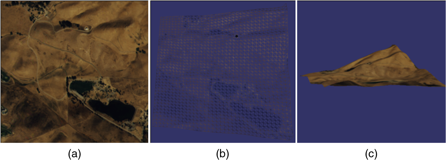

Second, the key bridge of an interaction algorithm between dynamic snow simulation and basal data is the 3-D terrain mesh. The accumulation of snow in our computing environment is calculated by the number of snow particles deposited at each grid in the terrain mesh. Based on the above deposit condition of snowflakes, it is not difficult to accurately obtain the accumulation. Obviously, real snow will change the visible color of the ground. In the simulation, what influences the snow will have upon the ground will depend on the type of the base ground data. In this article, we have used the hyperspectral remote sensing-image as ground data; snow particles deposited on the ground only impact hyperspectral remote-sensing data through visible effects or color changes. The interaction algorithm adopts a color-mixing calculation as shown below

In the above equation, ${\text{color}}_{\text{final}}$ is the final color of a ground pixel, ${\text{color}}_{\text{orgin}}$ is the initial color of the ground pixel, and $n$ is the number of snow particles in a quadrilateral mesh, where the ground pixel is located. ${\text{color}}_{\text{snowflake}}$ is the color increment of each snow particle. Assuming a $(r,g,b,a)$ values set is the representation of color, the color of pure snow is (1.0, 1.0, 1.0, 1.0), assuming a ground from pure black to pure white needs a deposit of at least 1000 snow particles; the incremental color value of each snow particle ${\text{color}}_{\text{snowflake}}$ is (0.001, 0.001, 0.001, 1.0). Eventually, the simulation result of a blizzard on the ground data is shown in Fig. 13.

Fig. 13

The snow simulation scene.

6.

Discussion

Dynamic simulations of geographical phenomena contribute to research and applications that fill the data blank between different temporal and spatial resolutions in remote sensing through computer technology. However, there has been a great deal of controversy regarding the method to conduct geological data simulation computing. Various studies have put forward suggestions for the internal drive of the phenomenon: 3-D data models and numerical algorithms.^3,20,21 We have focused on the simulation and interaction of snow with basal remote-sensing data. From the modeling and calculation work, we have concluded the general steps of geographical data evolution: which are summarized in the following sections.

7.

Conclusion

Remote-sensing data naturally have discontinuous time stamps because of the tracks of plane or orbits of satellites. In the foreseeable future, remote-sensing data will still be limited by discrete observation. Therefore, computational deduction that is based on remote-sensing data and the dynamic simulation of geological phenomena is a feasible but complex means to obtain spatial data of required specific spatial and temporal resolutions. On one hand, the dynamic mechanisms of geological phenomena are complex; on the other hand, a computational simulation of geological phenomenon involves many different fields. Nevertheless, we are seeking a methodology of geographical data evolution from a typical simulation process. Our detailed research on a snow scene with 3-D particle data model and hyperspectral remote-sensing data consists of a 3-D data model, snow simulation numerical, and ground remote sensing data interaction algorithms, and, eventually, remote-sensing data that are dynamically evolved in a virtual environment. Furthermore, we have extracted the general workflow and summarized the critical issues that arise from the simulation process and its result.

Thus, by using appropriate 3-D data models and a computational expression of geological, geographical, and environmental interactive phenomena, which reflects remote-sensing data, our methodology more closely predicts future Earth scenes and produces a better understanding of the multiscale environmental characteristics of the Earth than remote sensing alone. This methodology could also play an important role in critical tasks demanding data of specific spatial and temporal resolutions, especially in emergency response and rescue.