2.1.

Study Area and Imagery

In this study, Worldview-2 multispectral images were used for the image segmentation. Test image¹⁴ provides 11-bit data with a 0.50-m ground sampling distance and 8 multispectral channels (coastal blue, blue, green, yellow, red, red edge, near IR1, and near IR2). The data used in this study was segmented with Definiens Developer 7.0 software, and the segmentation quality parameters were calculated with ArcGIS software.

Our study area is located in the region Goričko, North-Eastern Slovenia (Fig. 1). The size of the area is $5\times 5{\mathrm{km}}^2$, and all five basic land-use classes are present: water, urban, forest, vegetation, and bare soil. The study area is mostly covered with intensive agricultural areas and there are just small villages and individual buildings; the forests are small, mainly islands in agricultural areas.

Fig. 1

Location of study area.

2.2.

Reference Data Set

For the evaluation of the segmentation, the supervised evaluation method⁴ is used. This method evaluates the segmentation by comparing the segmented image with a manually segmented reference image.⁴ The reference data consists of 89 manually segmented objects in the study area, i.e., 20 objects for each of the 4 basic classes (urban, forest, vegetation, and bare soil) and 9 objects for water. We collected just 9 objects for the class water because there are only a few objects in the study area that belong to this class and that are completely visible on the test image.

3.1.

Segmentation Quality Measures

Segments that overlap with the reference object by $>50\%$ were selected,^6,8 and the geometries of the segments that compose one reference object were calculated. Then selected segments were compared to the corresponding reference object and then the segmentation quality measures were calculated. The quality measures represent a measure of the discrepancies between the segmentation-based object and the reference object:⁵

Based on these measures, we can estimate the presence and shape agreement with the reference data.⁵ The measures for the estimation of the positional agreement were not included in this study. To facilitate a comparison between several segmentation results in the analysis, the normalized weighted segmentation quality measure, DQM (Ref. 5) was calculated. The optimal values and the weight for all the quality measures are determined for the calculation of the DQM, which is a weighted sum of the differences between the quality-measure value and the corresponding optimal value. The values of the weights and the optimal values are taken from Van Coillie et al.¹³ and are given in Table 1.

Table 1

Weights and optimal values for the calculation of the normalized weighted segmentation quality measure DQM based on four quality measures. Weights are taken from Neubert et al.9

Based on the four measures and the DQM, we evaluated the impact of the segmentation algorithm, its parameters, and the data resolution on the segmentation quality.

3.2.

Impact of the Segmentation Algorithm

The most suitable segmentation algorithms for multispectral or spatial information are covered by two types of algorithm, i.e., the edge-based algorithm, the region-growing algorithm, or a combination of the two.² In our analysis, we included one from each group, both of them integrated in Definiens Developer software (Ref. 15): the edge-based contrast split¹⁵ and the region-growing multiresolution algorithm.¹⁶

The purpose of the first group of analyses was to determine the optimal parameters of each segmentation algorithm. We estimated the optimal values of the parameters scale, shape, and compactness for the general case (independent of class object) and for the five land-use classes, i.e., water, forest, bare soil, vegetation, and urban. The scale parameter defines the maximum degree of homogeneity of the segments, and with this parameter we can determine the size of the segments; higher values allow more heterogeneity and result in larger segments. The parameter shape defines the influence of color (spectral value) and shape on the formation of the segments, while the parameter compactness defines whether the boundary of the segments should be smoother or more compact.

The parameter analysis of the multiresolution algorithm consists of 38 segmentations with a varying parameter scale (25, 50, 75, 100, 125, 150, 200, 300), compactness (0, 0.2, 0.5, 0.8, 1), and shape (0, 0.1, 03, 0.5, 0.7, 0.9). First, we keep the parameter scale constant and vary the parameters compactness and shape, with one of them always being kept constant.⁵ Then, we perform the parameter analysis of the contrast split algorithm, which is based on 29 segmentations with a varying parameter contrast mode (edge ratio, edge difference, and object difference), image layer (panchromatic, coastal blue, blue, green, yellow, red, red edge, near IR1, and near IR2), and chessboard tile size (20, 30, 40, 50, 60, 70, 80, 90, 100, 110, 150, 170, 200, 300, 500, 1000). In each segmentation group, we kept one parameter constant. Based on the segmentation-quality measures, we estimated the optimal parameters for both algorithms and compared the segmentation results using the multiresolution and contrast split algorithm with optimal parameters.

3.3.

Impact of the Spectral and Spatial Resolution

The digital values for different channels of the multispectral sensors can be correlated, which means that there is some redundant data in the multispectral images. This redundancy can be eliminated using principal component analysis (PCA), one of the transformations that reduce the correlation and the duplication of data while increasing the information density.¹⁷ The benefits of the PCA are:¹⁸ highlighting the characteristics of the image, image compression, and reducing the number of channels without a significant loss of information. The test image consists of 8 multispectral channels. We assumed that the data in individual channels are highly correlated and that using correlated data for image segmentation has a negative impact on the segmentation results. This assumption was proven with the segmentation of a transformed image using the PCA.

In the analysis of the spectral resolution, we used the multiresolution algorithm, which outperformed the contrast split algorithm in our segmentation algorithm analysis. To analyze the impact of spectral resolution, we performed a segmentation of a test image using 10 different combinations of the multispectral channels (Table 2) and the PCA transformed image.

Table 2

Impact of spectral resolution on segmentation quality. Acronyms for spectral bands are: R—red, G—green, B—blue, RE—red edge, CB—coastal blue, Y—yellow, PAN—panchromatic, NIR1—near IR 1, and NIR2—near IR 2. The data in the table is sorted using the DQM index from the lowest (best segmentation result) to the highest (worst segmentation result) value.

The purpose of last group of analyses was to investigate the impact of the spatial resolution. The higher spatial resolution results in more detailed objects on the image. With the analysis of the spatial resolution, we wanted to determine whether a high resolution gives us an advantage with respect to segmentation or not. The original image with a spatial resolution of 0.5 m was resampled to 2.5, 5, 10, 20, and 50 m. Due to the different spatial resolution, we re-estimated the optimal parameter values for each image separately and the segment images with the new optimal parameters.

4.1.

Multiresolution Algorithm

The purpose of multriresolution algorithm analysis is to assess the optimal parameter settings in the general case and in particular for objects belonging to the classes water, urban, bare soil, vegetation, and forest. We segmented the image with multiresolution segmentation, using different combinations of the parameters scale (25, 50, 75, 100, 125, 150, 200, 300), compactness (0, 0.2, 0.5, 0.8, 1), and shape (0, 0.1, 03, 0.5, 0.7, 0.9), where one parameter was always kept constant. The influence of the shape and compactness parameter settings on the segmentation result is shown in Fig. 2.

Fig. 2

Impact of shape and compactness parameter settings of the multiresolution algorithm on the segmentation quality is described with the segmentation quality index. The lowest values of the segmentation quality index mean the best quality of segmentation.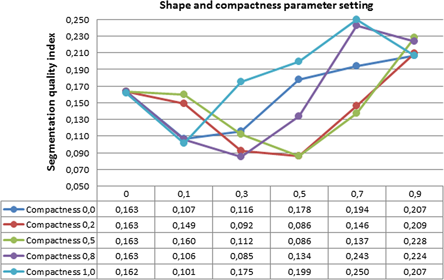

Based on all 38 segmentations runs, the best segmentation-quality measures for all five classes were reached for a shape setting of 0.3 and a compactness of 0.8, when we kept the scale parameter constant at 100. The graph in Fig. 2 shows that in the general case (objects of all classes), the worst segmentation results are achieved if the shape parameter is set to extreme values, e.g., 0 (color has the full influence on segmentation) and 0.9 (shape has the highest possible influence on segmentation). The results of the analysis show that the best segmentation quality is obtained if shape and color have a balanced influence on the generation of segments (the parameter shape is set to values from 0.3 to 0.5) and that the border of segments is not extremely smooth or compact (the parameter compactness is not set to extreme values, e.g., 0 or 1).

Table 3 shows the best parameter settings for all the classes in use and for the objects of a single class (urban, water, forest, bare soil, and vegetation). It is clear that the optimal parameter set of the multiresolution algorithm depends on the class that the objects belong to. The optimal setting of the scale parameter varies due to the different average size of the objects and the parameters shape and compactness vary because of the different properties of the objects belonging to the different classes. For example, the objects of the class urban (individual buildings) are small (and the parameter scale is set to the smallest value), and the objects of the class forest or bare soil are large (and the parameter scale is set to a higher value).

Table 3

Best parameter settings of the multiresolution algorithm for objects of the classes urban, water, forest, bare soil, and vegetation.

The data for the segmentation-quality measures in Table 3 show that using optimal settings for the algorithm parameters specific to a single class give better results than using the same parameters for all the classes. The exception is objects of the class water, because we run these tests based on RGB band combinations, and we should use additional spectral data to improve the segmentation quality of water objects. These tests are done in the next steps, while analyzing the impact of the spectral resolution on the segmentation quality.

If we consider the quality-measure values of single classes and of all five classes, we can see that we achieved a much better segmentation accuracy when we used the optimal parameters for a single class (except for the class water). Carleer et al.¹⁹ proposed multilevel segmentation, where one object class is segmented with its own set of parameters, according to the object’s characteristics. In order to prove that using specific parameter settings for objects of particular classes improve the overall segmentation accuracy, we performed classification-based segmentation. First, we performed a coarse segmentation of the test image using the multiresolution algorithm and classified the segments into five classes: urban, water, forest, bare soil, and vegetation. In the next step, we segmented the objects with the multiresolution algorithm using the best parameter setting (given in Table 3) and the best combination of spectral bands (given in Table 4) for objects belonging to one class. A comparison of classification-based segmentation and segmentation with one set of parameters for all objects is given in Table 5.

Table 4

Best spectral-band-combination settings for objects of a specific class.

Table 5

Comparison of classification-based segmentation and segmentation with one set of parameters.

The results in Table 5 show that classification-based segmentation produced better results than when using the uniform segmentation-algorithm settings for all the objects in an image, but at the expense of a higher average number of segments per object.

4.2.

Contrast Split

The purpose of the contrast split algorithm analysis is an assessment of the optimal settings of the parameters contrast mode, image layer, and chessboard tile size. We segmented the image with the contrast split algorithm using 29 different combinations of the parameters contrast mode (edge ratio, edge difference, and object difference), image layer (panchromatic, coastal blue, blue, green, yellow, red, red edge, near IR1, and near IR2), and chessboard tile size (20, 30, 40, 50, 60, 70, 80, 90, 100, 110, 150, 170, 200, 300, 500, 1000), where one parameter was always kept constant. In the test example, the setting for the parameter contrast mode has practically no influence on the result of the segmentation quality.

The segmentation with contrast split produced extremely over-segmented results, since the average number of segments composing one object was 98.5. But, on the other hand, very good matching of the shape and the area of the objects was achieved. The over-segmentation problem of the contrast split algorithm arises from the way in which the contrast is calculated. First, a high-resolution image is divided into equal square objects and then the split between bright and dark objects is performed.¹⁵ A detailed segmentation needs a large number of square objects, which results in a high shape accuracy, but also in an over-segmentation. We tried to reduce the number of segments by merging the spectrally similar segments together. The contrast split algorithm was combined with the spectral difference algorithm¹⁵ to eliminate the problem of over-segmentation. The number of segments was lower, but we did not succeed in drastically decreasing the average number of segments. In any case, the over-segmentation of all the other quality measures is very low, although extremely over-segmented results could cause serious problems in the classification step.

The contrast split algorithm uses just one spectral channel for segmenting the image. The impact of the selected spectral channel for the segmentation is analyzed in the next test. The segmentation-quality measures for all the spectral channels of the test image are given in Table 6.

Table 6

Impact of the of the setting parameter image layer on the segmentation-quality measures.

The best results in terms of segmentation quality (except for the number of segments) are achieved when using a red image layer and the worst results when using coastal blue or near IR bands.

A comparison of the contrast split and multiresolution algorithms is given in Fig. 3. The contrast split algorithm gives excellent results while segmenting objects of classes urban and bare soil. There is a very good matching of border and these objects are not over-segmented. However, for segmentation of forest, vegetation, and water, the contrast split algorithm indicated problems and the result is over-segmented. The boundaries of the objects are well defined, but there are many small segments inside the object. We tried to reduce the number of segments with the spectral difference algorithm, but we did not drastically decrease the average number of segments.

Fig. 3

Comparison of multiresolution (first row—a) and contrast split (second row—b) algorithm. Impact of the selected algorithm on the segmentation of objects belonging to the classes: urban (a1, b1), bare soil (a2, b2), vegetation (a3, b3), water (a4, b4), and forest (a5, b5).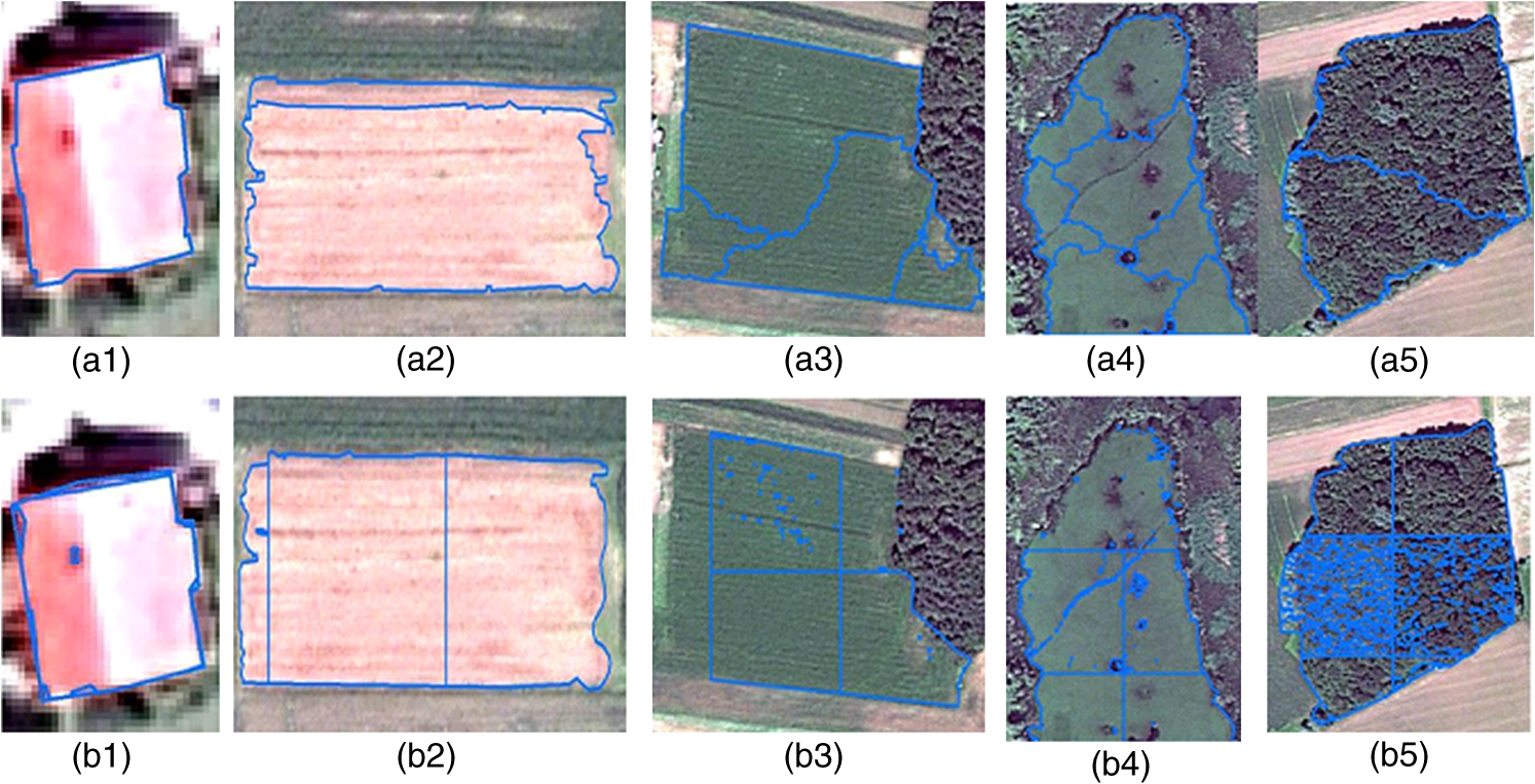

A comparison of the quality-measure values for both algorithms is given in Table 7. As mentioned before, the contrast split algorithm produces over-segmented results, but the difference in the area is lower (4.1%) than when using the multiresolution algorithm (6.9%). The difference in the perimeter is, in both cases, the same, and the difference in the shape index is lower when using the multiresolution algorithm.

Table 7

A comparison of quality-measure values for the contrast split and multiresolution algorithms.

Based on this comparison, we decided to use the multiresolution algorithm for an analysis of the impact of the spectral and spatial resolution on the segmentation quality.

4.3.

Impact of Spectral Resolution

The impact of the spectral resolution was investigated in order to find out whether a high spectral resolution improves the segmentation quality. The test image consists of a panchromatic and 8 spectral bands (coastal blue, blue, green, yellow, red, red edge, near IR1, and near IR2). The values on the different spectral bands are usually highly correlated,¹⁷ and we tried to remove this correlation with a PCA of the image; the first three components of the transformed image were used in the analysis.

We segmented the test image with the multiresolution algorithm and the optimal parameter settings (shape 0.3, compactness 0.8, and scale 100). In each segmentation cycle, we included a different combination of the spectral bands (Table 2) and the transformed image with the PCA.

Table 2 shows that worst results were achieved when using all 8 spectral bands and the best results when using just the red, green and blue bands. Segmentation based on all the spectral bands gave over-segmented results (average number of segments is 46.5), and the area difference was twice as high as when using just the RGB bands (13.5% versus 6.5%). The perimeter and the shape-index difference is, in both cases, nearly the same. The segmentation of the PCA-transformed image produces a result with a larger average number of segments (9.9), but all the other quality measures are the lowest (difference in area 5.8%, perimeter difference 2.5%, and difference in shape index 1.5%).

This result shows that a high spectral resolution and correlated data on different channels have a negative impact on the segmentation quality. With the PCA transformation, we removed the correlated data from the original image and achieved much better final results. This analysis demonstrates that high-spectral-resolution data is not an advantage for segmentation.

A comparison of the segmentation objects for specific classes based on the RGB bands, all the bands and based on the PCA-transformed image is given in Fig. 4. The biggest differences in matching the boundaries of the segmentation-based and reference objects are shown on the example of an urban object. The worst results are achieved when using all 8 spectral bands, and similar results are achieved when using a transformed image or when using the three original bands (RGB). In the case of other class objects, the best matching is achieved when using the transformed image, but with a larger average number of segments belonging to one reference object.

Fig. 4

Comparison of the segmentation of the RGB composite image (first row—a), original 8-multispectral bands WV-2 (second row—b) and transformed image with principal component analysis (third row—c). Examples of the segmentation of objects belonging to the classes urban (a1, b1, c1), bare soil (a2, b2, c2), vegetation (a3, b3, c3), water (a4, b4, c4), and forest (a5, b5, c5) are given.

Based on this analysis, the best spectral band combination is proposed for the objects of a specific class. For objects of the classes urban and forest, the best results are achieved when using the RGB bands; for the water classes it is recommended to add the RE band; and for bare soil objects it recommended to also add the near-IR1 band. Vegetation objects are specific in this case, because one vegetation object represents an area with one type of plant. In this case, we need a lot of spectral information to distinguish between the different species, so the best segmentation results are achieved when using 7 spectral bands (all the bands except coastal blue).

4.4.

Impact of Spatial Resolution

With the increasing spatial resolution of satellite images, it is possible to recognize more detail on the Earth’s surface. We analyzed the effect of the spatial resolution on the segmentation quality. Therefore, we downsampled the original image and prepared a series of images with spatial resolutions of 0.5, 2.5, 5, 10, 20, and 50 m. The images were segmented with the multiresolution algorithm and for each image an optimal value of the scale parameter was defined. The shape and compactness parameter values were constant at a shape of 0.3 and a compactness of 0.8. The impact of spatial resolution on the segmentation quality is shown in Table 8.

Table 8

Impact of spatial resolution on segmentation quality.

As described in the methodology section, the segmentation-quality measures are calculated based on overlapping segmentation-based objects and reference objects. From the segmentation layer, only segments that overlap reference objects by $>50\%$ were selected for the calculation of the segmentation quality.^6,8 In some cases, the reference object is represented only by one segment. If the overlap of the segment and the reference object is $<50\%$, this object is labeled as unrecognized. Therefore, by decreasing the spatial resolution of the image, the number of unrecognized objects rapidly increases (see Table 8). For the original spatial resolution, the number of these objects is 13, mainly objects of the class vegetation, where the segmentation did not distinguish between certain vegetation types. When increasing the spatial resolution to 2.5 m, the number of unrecognized objects increased tremendously to 61, and at 5 m and 10 m to 71. Decreasing the spatial resolution also increased the difference in the area, but the difference in the perimeter and shape index did not change.

The reference objects in this analysis are quite small and the original high spatial resolution is required to recognize all the objects in the segmentation process. Downsampling the spatial resolution drastically decreases the segmentation quality and the results of the segmentation based on downsampled images are not useful.

5.1.

Impact of Algorithm Selection

Two different segmentation algorithms, i.e., the multiresolution algorithm (region-growing method) and the contrast split algorithm (edge-based method) and their parameter settings were analyzed in detail. Both can produce a segmented image with a similar quality in terms of the differences in area, perimeter, and shape index, but at the expense of an extremely over-segmented result in the case of the contrast split algorithm. The average number of segments using the multiresolution algorithm is 2.3, while when using the contrast split algorithm it is 98.5. The over-segmentation problem of the contrast split algorithm arises from the way in which the contrast is calculated. We tried to reduce the number of segments by merging the neighboring segments with similar spectral values, but we could not drastically decrease the average number of segments. Based on an algorithm analysis we found the multiresolution algorithm to be more appropriate for the segmentation of high-resolution satellite images of Earth.

5.2.

Impact of the Algorithm Parameter Settings

We demonstrated that the multiresolution parameter settings have a great impact on the segmentation quality. We analyzed the parameter settings’ impact on the segmentation of an image in general and also the impact on objects of five classes (vegetation, urban, forest, water, and bare soil area) in particular. Furthermore, we demonstrated that each group of objects with similar characteristics should have its own set of optimal parameters for achieving the best possible segmentation result. Some objects have a characteristic shape and should have a high weight of the shape parameter; other objects do not have a characteristic shape, but are more determined by the spectral values and should have a high weight of the color parameter. The results of the classification-based segmentation proved that it is possible to achieve better segmentation results when using specific parameter settings and data selection for each class. Using class-specific segmentation parameters and data selection decrease the difference in area by 2%, the difference in the perimeter by 0.8%, while the difference in the shape index remains the same, i.e., 1.3%. However, using the optimal parameter settings as given in Table 5, produced over-segmented results. The average number of segments increased from 2.7 to 7.5.

5.3.

Impact of Spatial Resolution

The spatial resolution of the image has a very large impact on the quality of the image segmentation. Downsampling the image from 0.5 to 2.5, 5, 10, 20, and 50 m drastically decreased the quality of the segmentation results. Using a 2.5-m resolution instead of the original 0.5-m increases the number of unrecognized objects from 13 to 61. The objects are not recognized because they are represented by a segment that overlaps with the reference object by less than 50%. Moreover, decreasing the original spatial resolution to 2.5 m also increases the difference in the area by two times (from 6, 9 to 13, 4%). Reducing the spatial resolution makes sense in cases where the satellite image’s spatial resolution is too high in relation to the purpose of the object analysis. For example, a high-resolution image for mapping land use on a scale of 1:50.000 is too detailed. In this case, segmentation using an image with a low spatial resolution is recommended.

5.4.

Impact of Spectral Resolution

Spectral resolution also has a very large impact on the quality of the segmentation. The best segmentation results for the original image were achieved when using three spectral bands (red, green, and blue) and the worst results were achieved when using all 8 spectral bands. We estimate that the reason for the poor quality of the segmentation when using all 8 multispectral channels is the high correlation of the data in the different channels. The negative impact of the correlated data on the different spectral channels was demonstrated by a comparison of the segmentation of the original image with all 8 spectral bands and a PCA-transformed image, which removes the correlation between the data but maintains most of the information in the data.

The results of the unsupervised evaluation method show that we obtain much better segmentation quality using the PCA-transformed image. Using the transformed image instead of the original 8-MS-bands image decreases the average number of segments from 46.5 to 9.9, decreases the difference in the area from 13.5% to 5.8% and decreases the difference in the perimeter from 2.9% to 2.5%. Moreover, the results of the analysis show that with the PCA-transformed image we obtained even better results than when using just the red, green, and blue bands (the analysis shows that we obtained the best results with this original band combination). The red, green, and blue bands give a result with a smaller average number of segments, but all the other quality measures are better when using the PCA-transformed image (difference in area, perimeter, and shape index). The results of this comparison clearly show that using correlated and redundant data on different spectral channels decreases the segmentation quality. The biggest disadvantage of the PCA transformation is that each satellite image has its own transformation parameters. This drawback can be eliminated with the Tasseled cap (Kauth–Thomas) transformation, which has constant transformation parameters for the images of one satellite sensor. Unfortunately, the Tasseled cap transformation parameters for Worldview-2 have not been calculated yet. Therefore, the next step of this analysis would be a derivation of the Tasseled cap parameters and an evaluation of the segmentation quality of a transformed image with Tasseled cap. Future work will also include additional measures of the discrepancies that were not included in this study. An analysis of the positional differences between the segmentation-based and reference objects using different parameter settings, spectral, and data resolution will be carried out.

The analysis of the impact of spectral resolution on the segmentation of objects belonging to specific classes (urban, bare soil, vegetation, forest, and water) shows that for vegetation objects and water objects, it is possible to achieve a better segmentation quality using more than three bands (red, green, and blue). Objects belonging to the class vegetation are defined by the same type of crops. Broader spectral information is necessary to facilitate the identification of different types of crops, and the results of the analyses show that the best segmentation quality for vegetation objects is achieved when using seven multispectral channels (all except the coastal blue).

The spectral analysis of segmentation shows that less is more, since the use of low-spectral-resolution data provides a higher quality of segmentation. When operating with high-spectral-resolution data, it is therefore recommended to reduce the correlation between the data by using image transformations (for example, with a PCA).