1.

Introduction

Over the past several decades, optical remote sensing (RS) data has been widely used for evaluating changes in land-use dynamics,^1,2 biomass dynamics,³ and monitoring of degradation.⁴ At regional and national levels, vegetation indices have been commonly used to evaluate biophysical properties of forests. There are numerous examples of using optical RS for the study of land use, biomass, and degradation dynamics in tropical forests across the globe. The following sections will try to synthesize some of these.

Tangki and Chappell⁵ have evaluated the biomass variation in a selectively logged forest concession of Sabah by comparing field aboveground biomass (AGB) data with Normalized Difference Vegetation Index (NDVI) measures obtained from Landsat thematic mapper (TM) data. Results indicated that the NDVI explains up to 58% of the variation in AGB. However, the use of variables derived from optical RS data has had limited success in Borneo in predicting biomass.⁶ Ten vegetation indices were used in conjunction with field data to generate predictive relation for biomass estimations for a number of tropical sites, and these found weak correlations with field-based AGB measures.⁷

In addition to spectral-based methods using RS data, texture-based methods have provided valuable insights into the variation of forest structure, biophysical properties, and biomass dynamics in tropical forests of both Malaysia and Thailand.⁸ Research by Cutler et al.⁸ and Kuplich et al.⁹ using texture indices derived from high-resolution radar data has shown strong associations with AGB measures. Texture analysis of optical RS data has also been successfully used to quantify structural properties of forests.¹⁰ Wijaya et al.¹¹ used a number of Landsat-derived measures, including vegetation indices and texture variables, to examine spatial variations in AGB and forest stand parameters in Kalimantan. Their research has shown that the biomass and forest stand values have stronger associations with texture measures derived using gray-level co-occurrence matrices (GLCMs).¹¹ These findings have been corroborated by Ref. 12 using SPOT 5 data to derive spectral parameters and texture variables. Texture variables showed stronger associations with forest stand parameters, such as basal area, bole volume, and canopy height, than with spectral parameters.

These examples illustrate that the spectral characteristics of optical data (such as vegetation indices) have been widely used for studying biomass dynamics, but their performance has been limited to explain forest biophysical parameters in dense tropical forests. Texture analysis (such as those derived from GLCM) is a promising alternative to characterize the variation in AGB and forest stand parameters. However, these techniques have so far not been tested on landscapes dominated by oil palm plantations containing isolated forests such as riparian forest (RF) zones.

2.

Rationale and Objectives

Logging, deforestation, and conversion of land to oil palm plantation have increased forest fragmentation in Borneo. Given the extent of forest loss and logging, it is essential to evaluate the ability of remnant forests to provide AGB storage and retention of tree biodiversity, especially forest fragments and riparian margins. A riparian forest zone (RF) is defined as the land adjacent to streams and rivers. Malaysia has 189 river systems, out of which 78 are located in Sabah. Riparian zones are legally protected and should be maintained for all permanent water courses. The width of these buffer zones varies according to state laws.¹³ In the riparian zones of the study area, a width of 30 m on each side of the waterway has been retained in all forest types.¹⁴ A significant body of literature indicates that the presence of RFs in a landscape can assist in biodiversity conservation.^15,16 However, despite legal protection, RF zones are vulnerable to illegal logging.¹⁷ Currently, there are no frameworks in place to identify RF zones at the landscape scale and to monitor the variation in AGB stocks. Optical RS imageries, such as Landsat and SPOT, are widely available for free or at low cost. The motivation behind the present study is to identify techniques (such as vegetation and texture indices) which could be applied to these widely available dataset and would allow for monitoring the impacts of logging and the identification of isolated forest zones in mixed landscapes such as those found in Borneo. It is anticipated that this type of research could inform RS-based monitoring of oil palm tropical forest landscapes and smaller isolated forests located within these landscapes.

The objectives of the present study are: (a) to examine whether it is possible to distinguish between old growth primary forests, RFs of different logging intensities, and oil palm plantations using the spectral characteristics of Landsat TM and SPOT 5 data, (b) to examine whether texture-based measures can provide insights into the spatial variation of forest structure and biomass dynamics across the different forest types, and (c) to generate biomass estimation models of the study area using RS data. To accomplish these objectives, several image-processing techniques are employed to enable the detection and mapping of land-cover patterns and to generate biomass estimation models for the different land-use types.

3.

Methodology

3.1.

Study Area

The research was carried out at the study site of the Stability of Altered Forest Ecosystems (SAFE) Project located in the Yayasan Sabah Concession area^14,18 in Sabah, Malaysia (Fig. 1). The area consists of a mixed landscape that includes areas of a twice logged forest virgin jungle reserve (VJR), oil palm plantations (OP), and a 7200 ha heavily logged area known as the experimental area (EA), which has been ear marked for the conversion to oil palm plantation beginning in December 2011. The study area extends to the Maliau Conservation Basin (116.87 E, 4.82 N). It has been proposed to retain circular arrangements of forests (of varying forest cover). A number of RF sites will also be retained both in the proposed and in the existing oil palm plantations. In addition, RF zones will be retained in other land-use types.

Fig. 1

(a) Location of Sabah in Borneo. (b) Location of the study area within Sabah.¹⁸

Based on ground-truth data provided by SAFE, several different land-use types are present in the study area.¹⁴ These include old growth primary forests (OG), disturbed forests (which have been exposed to slight anthropogenic disturbance and clearance), VJR (which have been logged once at most), twice logged forests (LF), heavily logged forests (EA; which have undergone three rounds of logging and are in a state of severe degradation), RFs, and oil palm plantations (OP). Details of the structures of the various forest types in study area are presented in Table 1. These different forest types have significant differences in their stand and canopy structure (see Tables 2 and 3).

Table 1

Structure of different forest types present in the study area (photographs taken at the SAFE project site, 2011).

Land-use categories	Illustrative photograph
Old Growth Forests (OG) These are pristine lowland forests located in the MBCA. The slope of these forest locations does not exceed 20 deg. These forests are characterized by a closed canopy and the presence of very large Dipterocarp trees. Some of the trees have heights of $>50\mathrm{m}$ and diameter at breast height (DBH) of $>80\mathrm{cm}$. Tree species survey was carried out and it revealed that these forests also host IUCN red listed Endangered Dipterocarp species such as Shorea johorensis. These forests also have a very thick understory
Oil Palm Plantations (OP) The SAFE project site contains oil palm plantations with ages ranging from 5- to 8-years old. Oil palm plantations are characterized by a homogenous canopy structure and negligible tree species diversity. The picture shows the aerial view of the oil palm plantations in Sabah19
Heavily logged forests (EA) These are highly degraded forests, which have undergone several rounds of logging. These are characterized by the presence of large open areas and broken canopy. Virtually no large trees are observed, and the area is dominated by small successional trees and ginger shrubs
Riparian forests (RF) These are forest zones adjacent to rivers and streams. These are dominated by thin and tall vegetations and trees of the Maccaranga genera. In some of the riparian zones, the evidence of illegal logging has been observed based on to the presence of logging tracts. These forests are relatively intact compared with the surrounding heavily logged and twice logged forests

Table 2

Aboveground forest parameters across the riparian forests (RF).

	${(\mathrm{OG})}_{\mathrm{RF}}$	${(\mathrm{VJR})}_{\mathrm{RF}}$	${(\mathrm{LF})}_{\mathrm{RF}}$	${(\mathrm{EA})}_{\mathrm{RF}}$	${(\mathrm{OP})}_{\mathrm{RF}}$
Basal area (${\mathrm{m}}^2/\mathrm{ha}$)	$56.28\pm 9.27$	$55\pm 8.1537$	$49.75\pm 9.19$	$29.146\pm 5.52$	$34.183\pm 3.205$
Basal area of trees with $\mathrm{DBH}>10\mathrm{cm}$ (${\mathrm{m}}^2/\mathrm{ha}$)	$55.8\pm 8.878$	$54.486\pm 7.98$	$48\pm 9.74$	$25.289\pm 5.18$	$32.44\pm 3.18$
Tree height (m)	$19.7\pm 0.83$	$18.9\pm 1.31$	$22.7\pm 1.44$	$9.2\pm 0.33$	$9.7\pm 0.25$
Stem density (/ha)	667	714	629	840	1056
Stem density of trees with $\mathrm{DBH}>10\mathrm{cm}$ (/ha)	488	481	456	440	601

OG: Old growth forests; VJR: virgin jungle reserve; LF: logged forest; EA: experimental area; OP: oil palm plantations.

Table 3

Aboveground forest parameters across the non-RF (NRF) zones.

	${(\mathrm{OG})}_{\mathrm{NRF}}$	${(\mathrm{VJR})}_{\mathrm{NRF}}$	${(\mathrm{LF})}_{\mathrm{NRF}}$	${(\mathrm{EA})}_{\mathrm{NRF}}$
Basal area of trees with DBH $>10\mathrm{cm}$ (${\mathrm{m}}^2/\mathrm{ha}$)	$65.39\pm 3.1$	NA	$32.13\pm 13.43$	$17.14\pm 2.17$
Stem density of trees with DBH $>10\mathrm{cm}$ (/ha)	820	NA	592	417

Data for forest mensuration parameters across different land-use types [diameter at breast height (DBH)] was obtained using 193 ($25\times 25{\mathrm{m}}^2$) vegetation plots spread across the different forest types in the study area.¹⁴ These vegetation plots have been set up following a fractal design.²⁰ In the RFs of each of the different forest types, six plots ($10\times 50{\mathrm{m}}^2$) were set up in three riparian zones each. For each forest type, 18 plots were established from September to December 2011. Plot establishment followed a random stratified sampling strategy. The plots are located in all forest types present in the study area, but within each study area, they have been located randomly. In riparian plots, both DBH and tree height (H) were measured. Table 2 presents the forest mensuration variables measured from both riparian and non-riparian plots of different land-use types.

Tree heights for non-riparian plots were estimated using a DBH-height relationship provided by Ref. 21. The AGB of the trees in both riparian and non-riparian zones was calculated using the biomass equation recommended by Ref. 22

Eq. (1)

$$\text{Aboveground}\text{Biomass}(\mathrm{AGB})=0.0776\times {(\rho \times {\mathrm{DBH}}^2\times \mathrm{H})}^{0.94},$$

where $\rho$ refers to the wood-specific gravity. Given the difference in the physiology of oil palm trees and regular forest trees, specific biomass equations are needed to calculate the AGB of oil palm plantations. The AGB of oil palm trees was calculated using the biomass equation recommended by Ref. 23

Eq. (2)

$${(\mathrm{AGB})}_{\text{Trunk}}=100\times \pi \times {(r\times z)}^2\times h\times \rho ,$$

where $r$ is the radius of the trunk (in cm) without frond bases, $z$ is the ratio of the trunk diameter below the frond bases to the measured diameter above the frond bases (estimated to be 0.777 from the sampled trunks), and $h$ is the height of the trunk (in m) to the base of the fronds. The trunk density $\rho$ (in $\mathrm{kg}{\mathrm{m}}^{-3}$) is defined as follows:

Eq. (3)

$$\rho =(0.0076x+0.083)/100,$$

where $x$ is the age of the oil palm plantation.

4.

Results

4.1.

Land-Cover Map of the Study Area

The land-cover map of the study area (Fig. 2) was created using Landsat TM data and clearly delineates the areas of different logging intensities in the study area along with the areas of primary forest, oil palm plantations, and logged forests.

Fig. 2

Landsat TM-derived land-cover map of the study area. Gray lines represent the SAFE and Maliau basin conservation area (MBCA) boundaries.

While most of the field survey data were used for generating training pixels or regions of interest (ROIs), 30% of the field survey data was set aside for validation. A confusion matrix was used to describe the accuracy of the classification.³² The classified Landsat image had a classification accuracy of 77% and a kappa coefficient of 0.45.

4.2.

Distinguishing Between Different Land-Use Classes Using Reflectance and Vegetation Indices

4.2.1.

Efficacy of SPOT 5-based RS data in distinguishing between different land-use types

Band reflectance and spectral-based vegetation indices were used to distinguish between the different forest types in the study area (Fig. 3). All forest-use types show substantial differences in the shortwave band of the SPOT data. While other bands, such as infrared and red bands, can distinguish between the major forest classes, they cannot distinguish non-riparian zones from riparian zones and twice logged forests from heavily logged forests. All three bands can distinguish oil palm plantations from other forest types. However, the different logged forests show overlap in the red and NIR bands.

Fig. 3

SPOT-derived vegetation indices for different land-use types. OG: old growth forests; OP: oil palm plantations; RF: riparian forests; VJR: virgin jungle reserve; EA: experimental area; and LF: twice logged forests.

Vegetation indices derived from the higher resolution SPOT data were used to distinguish between different forest types present in the study area. The values for NDVI and NDII5 decrease sharply from primary forests to once logged forests and then increase from once logged to twice logged to heavily logged forests. The NDVI values based on SPOT 5 are able to distinguish between different forest types and forest transition systems in the study area. The NDVI values differ significantly between old growth primary forests, once logged forests, twice logged forests, and heavily logged forests. The oil palm plantations can also be distinguished from all other land-use types. However, NDVI was not able to distinguish between the RFs and the pristine, once logged, and twice logged forests. The NDVI values differ significantly between heavily logged forests and oil palm plantations. However, SAVI is not as effective in distinguishing between different forest types. The SAVI values varied significantly between the old growth pristine forests and once or slightly logged forests and old growth forests and heavily logged forests. However, SAVI values did not differ significantly between the once logged, twice logged, and heavily logged forests. The SAVI values (like NDVI) differ significantly between oil palm plantations and all other forest transition systems. The NDII5 is not able to distinguish oil palm plantations from other land-use types.

4.2.2.

Efficacy of Landsat TM-based RS data in distinguishing between different land-use types in the area

Based on Landsat TM data, NDVI values differ significantly between oil palm plantations and other land-use types. However, NDVI values cannot distinguish between forests that have undergone different logging intensities. These results can be attributed to the saturation of the NDVI value at high biomass levels.^33,34 This limits their ability to predict biomass in tropical forests such as those in Borneo.

4.3.

Correlation Between VIs and Field Measures of AGB

Predictive models of biomass were generated using AGB data collected using field surveys in conjunction with vegetation indices and band reflectances derived from Landsat TM and SPOT 5 data. Reflectance values of the green (band 1), red (band 2), NIR (band 3), and SWIR (band 4) bands of the SPOT 5 data were correlated with field-based AGB data to derive biomass estimation models. The biomass estimation model is as follows:

Eq. (7)

$${(\text{Biomass})}_{\mathrm{SPOT}}=106.37*(\text{Band}1)-33.72*(\text{Band}2)+124.33*(\text{Band}3)+40.73*(\text{Band}4)-\mathrm{130.71.}$$

A strong association was found between field-based AGB values and those derived using all of the SPOT bands. However, the SPOT biomass model in Eq. (7) tends to underestimate the AGB values. While most of the field-based AGB data were used to establish the coefficients in Eq. (7), a sample of the data was set aside for validation purposes. The results of validation are presented in Fig. 4. A biomass estimation model using the red, NIR, and SWIR bands also displays a high correlation ($R^2=0.8512$, $p<0.001$) with field-based AGB values. Single-band biomass estimation models consisting of red (band 3) and NIR (band 4) bands have an $R^2$ value of 0.80 and 0.833, respectively ($p<0.001$).

Fig. 4

Actual and expected regression models between AGB values derived using SPOT imagery and field observations. All four SPOT bands (green, red, NIR, and SWIR) were used for deriving SPOT-derived AGB.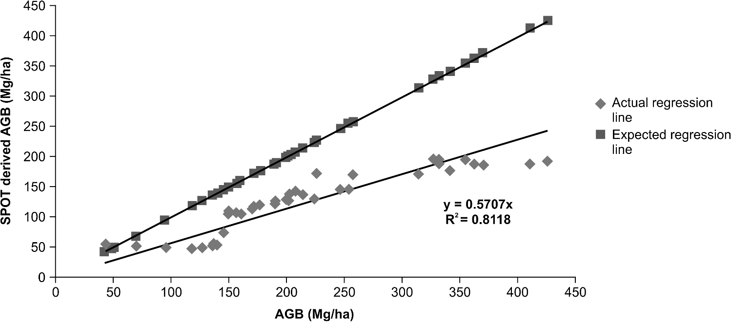

Based on Landsat data, NDVI has a very weak correlation ($R^2=0.0562$, $p<0.01$) with the field-based AGB values. Other vegetation indices, such as SAVI, also show a very weak correlation with the field-based AGB values. On the other hand, the reflectance values of band 3 show a strong association with the field-based AGB values ($R^2=0.85$, $p<0.01$), whereas the correlation is weaker for band 4 ($R^2=0.59$, $p<0.01$). The biomass estimation model based on band reflectance value can be expressed as

Eq. (8)

$$B_{\mathrm{a}}=-2175.4(\text{Band}4)+2628.3$$

Eq. (9)

$$B_{\mathrm{a}}=-2776(\text{Band}3)+2817.4,$$

where $B_{\mathrm{a}}$ is the mean biomass of study area (in $\mathrm{Mg}/\mathrm{ha}$), which has been obtained from the reflectance values of bands 3 and 4.

4.4.

Use of Texture-Based Variables in Evaluating Forest Stand Parameters and Biomass Dynamics

High-resolution satellite data is better suited for the calculation of texture indices than coarse- and medium-resolution data.^28,35 For this reason, comparatively higher resolution SPOT data is used for obtaining the texture-based variables. Two vegetation attributes are employed: AGB and basal area. A statistical examination of the AGB values in the different land-use types indicates that they are influenced by the disturbance due to several rounds of logging and oil palm cultivation. Regression models were generated to describe the relationships between the vegetation attributes and the texture variables described in Table 4. The texture variables showed strong but varying associations with AGB and basal area of the different forest types (Table 5).

Table 5

Ability of texture-based linear regression models to explain variation in vegetation attributes.

Forest type	AGB	Basal area
EA	$R^2=0.86$ ($p<0.01$)	$R^2=0.92$ ($p<0.01$)
LF	$R^2=0.88$ ($p<0.01$)	$R^2=0.72$ ($p<0.01$)
VJR	$R^2=0.90$ ($p<0.01$)	$R^2=0.98$ ($p<0.01$)
RF	$R^2=0.91$ ($p<0.01$)	$R^2=0.84$ ($p<0.01$)
OP	NA	NA

However, the results for oil palm plantations were not significant. The texture-based biomass estimation models (which were built using the variables mean, variance, and contrast) underestimated the AGB values for all the land-use types considered. The validation results for some of the land-use types are presented in Fig. 5.

Fig. 5

(a): Comparison between Field and Texture derived AGB for EA (b) Comparison between Field and Texture derived AGB for LF (c) Comparison between Field and Texture derived AGB for RF. In all three cases, it can be seen that while there is strong relationship between field and texture AGB, texture based AGB values underestimate field AGB values for all three land use types under consideration.

5.

Discussion

The present study compares a number of RS variables that can be used for the evaluation of land use and biomass dynamics. The research has accomplished two out of its three objectives. The first objective was to use vegetation indices and band reflectance values derived from Landsat and SPOT data to distinguish between different forest types in the study area. The results indicate that the vegetation indices derived from Landsat TM and SPOT 5 data have a limited potential to distinguish between the different land-use types. Vegetation indices derived from Landsat data (such as NDVI) can distinguish between major land-use types, such as old growth pristine forests and oil palm plantations, but not between forests with different logging intensities. The NDVI derived from higher resolution SPOT data can distinguish between pristine forests, forests of different logging intensities, and oil palm plantations. However, other SPOT-based vegetation indices also cannot distinguish between forests of different logging intensities. In addition, vegetation indices derived from both Landsat TM and SPOT 5 (such as NDVI) are not strongly correlated with the field-based AGB values. For the particular study area, the vegetation indices are insufficient for distinguishing between forests of different logging intensities and for generating biomass estimation models for individual land-use types. This confirms the growing body of literature which indicates that the use of spectral information is limited due to its saturation at high biomass values, thereby restricting its utility.^{7,11,12,26,31,36} As opposed to the vegetation indices, reflectance values of bands 3 and 4 of Landsat are strongly correlated with the field-based AGB values. Similarly, strong associations have been observed in a logged forest-pristine forest study site (similar to ours) located in the Danum Valley Conservation Area, which is close to the SAFE study area.⁵

The second and third objectives were to use texture-based variables to examine the structure and biomass parameters of different forest types in the study area and to evaluate the possibility of developing biomass estimation models for the different forest types. The use of the GLCM-based texture analysis methods provides insight into the biomass and structural dynamics across different land-use types. The texture analysis also helps identify that the different land-use types, including forests having undergone different logging rotations, vary in terms of their structure. Optical RS data can be used to identify (and delineate) small fragmented areas such as riparian zones and forests having different logging intensities. Statistically based texture variables have been widely cited in the literature for their strong association with variation in forest structure, forest stand parameters, and biomass dynamics.^8,11,31 This accomplishes the second objective of the research. Table 5 shows that the regression models using texture variables and field-based AGB values vary for different forest types in terms of their strength. It can therefore be concluded that the use of texture analysis opens up the possibility of developing different biomass estimation models for different land-use types. This accomplished the third objective of the research.

In summary, the present study confirms the findings of previous research that vegetation indices derived from optical RS data have limited potential to distinguish between different forest types compared with texture-derived measures. The present study has determined that AGB is underestimated by both spectral and textural variables. A possible reason for this could be biomass saturation. This suggests that optical RS biomass estimation models need to be interpreted with care. Most importantly, however, the present study has shown that it is possible to identify isolated RF zones and to show that their structure and biomass dynamics differ from surrounding logged forests. To the best of our knowledge, only one field-based study has previously been carried out on the RFs of Malaysia.¹³ Arguably, texture-based analyses could be applied for studying the biomass and structure dynamics of isolated forest fragments.

6.

Conclusions and Future Directions

The RS data offers the potential to study various forest properties including their structure, carbon dynamics, and assessment of degradation. The present study has shown a number of different techniques that may be used to overcome the shortcomings of optical RS data. Most importantly, the efficacy of these different techniques in examining the structural and biomass dynamics of tropical forests has been demonstrated, especially in the case of mixed land-use types. This research can be applied to the management of lowland Dipterocarp forests and to the evaluation of their carbon stocks. The present study has established that the band reflectance and texture measures derived from GLCM can be used to generate biomass estimation models that correlate strongly with the field-based AGB. The biomass estimation models derived from texture variables can be applied to similar mixed land-use types. Application of these biomass estimate models could allow for the assessment of timber stocks and for the assessment of the ecological status in terms of forest recovery and variation in carbon stocks. Most importantly, the use of biomass estimate models makes it possible to examine both the spatial variation in forest canopy structure and carbon stocks across a variety of different land-use types and disturbance gradients. Texture analysis of optical RS images is a very promising technique for a study area like Borneo, where traditional vegetation indices-based analysis may be limited due to data saturation for sites with high biomass density or sites having complex forest stand structure.³⁷