|
|
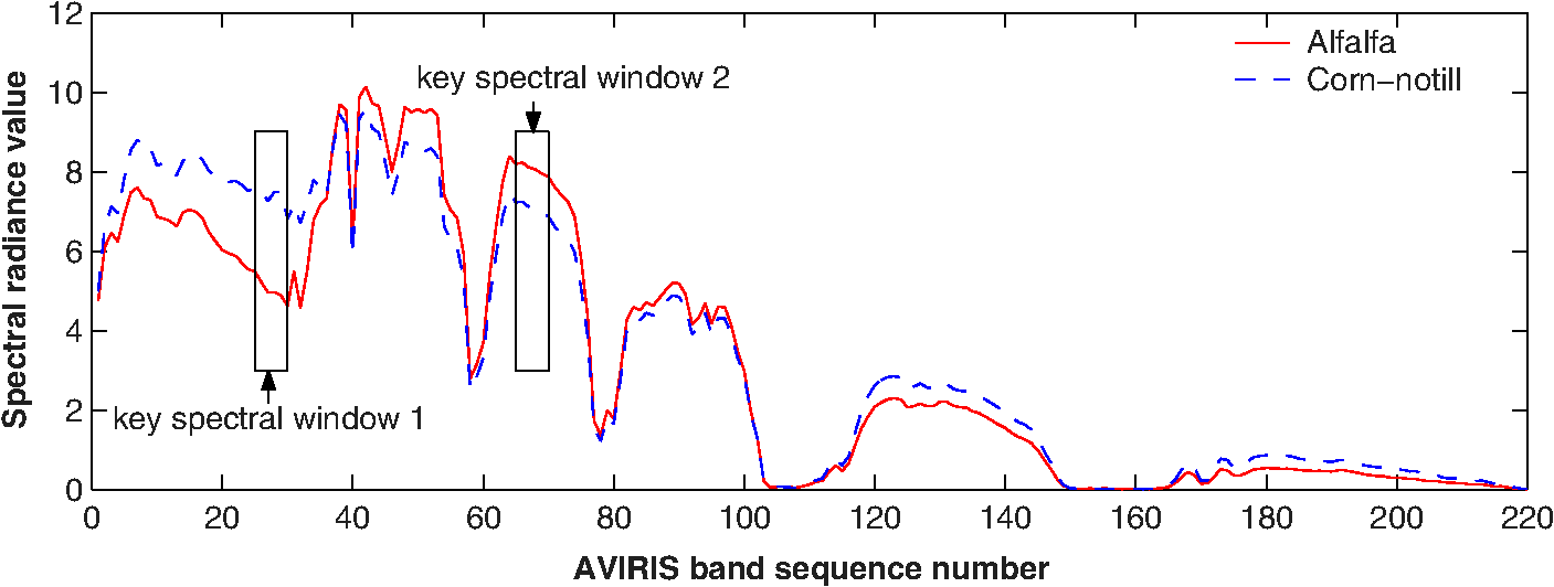
1.IntroductionHyperspectral sensors simultaneously measure hundreds of contiguous spectral bands with a fine spectral resolution, e.g., 0.01 μm. This makes it possible to reduce overlap between classes and, therefore, enhances the potential to discriminate subtle spectral difference.1,2 Using data from hyperspectral sensors, classification is carried out by analyzing the electromagnetic reflectance as a function of the wavelength or band, i.e., the spectral signature. In recent years, hyperspectral image classification has received significant attention in many applications.3–5 However, the large number of spectral bands also presents several significant challenges to hyperspectral image classification. First, an increased number of spectral bands means a higher dimensionality of hyperspectral data. For instance, the AVIRIS hyperspectral sensor6 has 224 spectral bands ranging from 0.4 to 2.5 μm, and the original signal is 224 dimensional. It is known that the high dimensionality of input space would deteriorate the performance of many classification methods7 if no appropriate preprocessing is applied. Second, although there may be hundreds of bands available for analysis, not all bands contain the essential discriminatory information for classification. In the wide spectrum, it is to be expected that different parts of the spectrum will have differing representative capabilities to distinguish the objects of interest. In some parts of the spectrum, materials may have a much more unique spectral response than other parts of the spectrum. Finally, the high dimensionality inevitably results in a larger volume of data. Whether using conventional classification algorithms or modern methods, the requirements for storage space, computational load, and communication bandwidth are factors that have stringent constraints, particularly in real-time applications. To limit the negative effects incurred by higher dimensionality, it is advantageous to remove parts of the spectral bands that convey less discriminatory information. In the past, many band selection techniques have been proposed, such as search-based methods,8–10 transform-based methods,11,12 and information-based methods.13–15 Other band selection techniques include a trade-off scheme between the spectral resolution and spatial resolution,16 maximization of spectral angle mapper,17 high-order moments,18 and wavelet analysis.19 However, there are still some challenges to apply this technique effectively, such as higher computational cost, suffering of local minimal problems, loss of the original physical meaning, difficulties for real-time implementation, etc. In this research, we study the band selection in the context of data classification, where retaining raw data appearance and not losing the original physical meaning are desirable for the purpose of registration with other source images [e.g., synthetic aperture radar (SAR) imagery]. In this case, the dimensionality-reduction techniques based on feature selection is particularly attractive. As derived from the concept of entropy, mutual information (MI) measures the statistical dependence between two random variables and, therefore, can be used for feature selection. Although entropy10,13 and MI (Refs. 11 and 20) have obvious potential for band selection, this has not been fully exploited in the past. In Ref. 21, MI has been used to increase the radiometric resolution or signal-to-noise ratio. In our previous research,14,15 a heuristic approach has been proposed, where the estimation of MI was based on domain experts’ subjective judgment. The simulation in Ref. 14 showed favored results for the MI-based method compared to the other three representative competitors (namely the steepest ascent searching method, the entropy-based method, and the correlation-based method). As a supervised feature selection method, one of the main obstacles regarding the MI-based approach is its reliance on availability of a reference map (i.e., the ground truth map, in which each pixel is correctly labeled by its class). To obtain a full reference map, expensive ground survey and manual labeling are usually involved, which put prohibitive factors to apply this technique in practice. To improve the applicability of the method, we propose a new band-selection scheme based on estimating a reference map, which is constructed by Parzen window approximation and optimization algorithms. In the proposed method, the reference map is estimated by using a group of bands with a higher separability. Because the high-separability bands are likely to appear in a spectrum, where the light is absorbed by the constituent atoms or molecules,22 bands in these characteristic regions are more useful to classification and they are contiguous naturally. It is, therefore, desirable to make a continuous constraint for the bands used to estimate the reference map. In other words, a spectral window can be built to capture the bands in the particular spectrum. Other two advantages are reducing counteraction of discriminatory information among bands and avoiding the increase of computational cost, which will be discussed in the end of Sec. 2. Experiments are carried out to evaluate the effectiveness of the proposed method using a public hyperspectral dataset AVIRIS 92AV3C and a high spatial resolution dataset “Pavia University scene.” The results show that the proposed method can remove a significant amount of redundant bands without significant loss of classification accuracy. The remainder of this paper is organized as follows. In Sec. 2, we discuss the band selection method based on the MI analysis. In Sec. 3, we propose the new MI-based band selection scheme. Experimental results are reported in Sec. 4. Finally, we end this paper with conclusions. 2.Hyperspectral Band Selection Through Mutual Information AnalysisMI is a basic concept in information theory to measure the statistical dependence between two random variables.23,24 Given two random variables and , with marginal probability distributions and , and joint probability distribution , MI is defined as According to Shannon’s information theory, entropy measures information content in terms of uncertainty and is defined by From Eqs. (1) and (2), it is not difficult to find that MI is related to entropies by the following equations: where and are the entropy of and , is their joint entropy, and and are the conditional entropies of given and of given , respectively. The joint and conditional entropies can be written asIf we treat the pixels’ value in a spectral band as a random variable and their corresponding value in the reference map as another random variable, MI between them can be used to estimate the dependency between this spectral band and the reference map. This is helpful to investigate how much common information a spectral band contains about the reference map. Since the reference map represents the class label of each pixel and implicitly defines the required classification result, the above MI measures the relative utility of each spectral band to the classification objective and can be used to select bands. A weakness of the straightforward MI-based band-selection method is its reliance on a reference map. The reference map is usually obtained from a ground survey or manual labeling by domain expert, which is always costly and time-consuming. In many practical applications, a complete reference map is simply not available. To improve the applicability of the method, we propose a new band-selection scheme based on estimating a reference map. In this case, instead of calculating the MI based on the reference map, , an estimated reference map, , is used. This is assumed to be easy to obtain and to be a good estimate of . In details, the estimated reference map is calculated using a group of spectral images, i.e., key spectra , which are assumed to have the best discriminatory capability. So, if , are images from the set of key spectra ; then the estimated reference map is obtained as The advantage of using a number of bands, rather than a single spectral band, to estimate the reference map is to average out the possible noise and reduce uncertainty. Moreover, it is preferable that these bands are contiguous in the spectrum. The proposed spectral window is designed to capture bands with a higher separability for classification. It is known22 that the high separability is likely to appear in the spectrum where certain atoms or molecules (of which the material is made of) absorb the light. Apparently, bands contained in these particular regions are contiguous. The second reason to keep the bands contiguous is if these bands are not adjacent, the intensities of their pixels may counteract each other. Figure 1 gives an example where two groups of bands, labeled as the key spectral spectra 1 and 2, were found with the most discriminatory information. Because the intensity priority is inversed for these two regions, directly averaging their spectral responses may lose rather than enhance discriminatory information. The third reason is to avoid the increase of computational cost that will happen when a group of separated bands are selected (e.g., the combinatory explosion). Based on a metric of goodness, the key spectra can be found by a searching algorithm, which is presented in Sec. 3. 3.Constructing an Optimal Estimate of the Reference MapA hyperspectral imagery can be considered as an image cube (see Fig. 2) where two axes are spatial dimensions (i.e., the coordinates of the observed scene) and the third axis is the spectral dimension (i.e., the spectral channels or bands). As we discussed in Sec. 2, to estimate the reference map, we need to find a group of most informative bands and make sure that their reflectance intensities do not counteract each other. This problem can be modeled as a procedure of seeking an optimal spectral window along the spectral dimension in the hyperspectral data cube (see Fig. 2). By controlling the width of the spectral window, we can keep the bands within the window positively correlated (i.e., no intensity inverse) and avoid the offset of discriminatory information. It should be noted that in the whole images, different local areas may present different trend in correlation. However, only when different areas show the same positive correlation within the spectral window, averaging these bands can reduce noise or uncertainty and, therefore, increase the reliability to approximate the ground truth. So if a compensation effect between positively and negatively correlated areas occurs, the resulting estimated reference map will be less accurate. According to the searching algorithm introduced in Sec. 3.3, this spectral window will not be chosen as a final solution and a next step of searching will be incurred until a better spectral window is found. 3.1.Model of Spectral WindowGiven a hyperspectral feature vector , each component denotes a spectral reflectance or radiance value measured at the band , . is the total number of spectral bands in a spectrometer. This number could be as many as 200 for a normal hyperspectral sensor. Given that is a transform that can choose a subset of contiguous bands at the spectrum position within a -width window, is a chunk of spectral signal within the spectral window (see Fig. 2). where represents the subset bands within the spectral window specified by the parameters and . By shifting the spectral window forward or backward along the spectral axis, we are able to evaluate the discriminatory capability for each group of contiguous bands and then find the optimal subset of bands to approximate the ground truth. This problem can be formalized as follows: where is a metric of goodness of a chunked feature vector to approximate the class label . Thus, the continuous spectral bands that we are looking for are given byTo automatically find the best spectral window, we may consider MI as a metric . As long as the derivative of this MI is known, we can decide how the spectral window should move, i.e., the gradient ascending algorithm. For other similarity metrics, such as correlation or spectral angle, it is not so easy to find their analytic expression and apply them to the gradient-based algorithms. According to Eq. (3), the MI can be written as We can see that the MI described in the right side of the first row of Eq. (10) has two terms. The first one is the entropy of the class label variable . It is not a function of the window-shifting transform . The second term is a conditional entropy of given the chunked spectral feature vector . When the class label variable and the chunked spectral feature vector are related, the amount of entropy, , will reduce. For example, if can be predicted by reliably, then will become less uncertain when we have the observation of . If we intuitively understand the entropy as the amount of uncertainty, the decrease of uncertainty means less of entropy. In other words, if is a good observation or informative feature subset to predict the unknown variable , the uncertainty of will reduce more than other less discriminatory feature subsets. As a result, will decrease. From Eq. (10), the less amount of will increase the MI, . Consequently, considering that , maximizing the MI in Eq. (10) will encourage the spectral window to shift to a wavelength region in which the spectral features would have a better capability to predict the class label. Also, there is a bound relationship between the MI and the Bayes error,25 so the bands subset found by Eq. (8) would have a good discriminatory capability for classification in the sense of Bayes error. In the following paragraphs, we discuss how to obtain the differentiable MI to maximize . 3.2.Differentiable Mutual InformationIn Eq. (10), the MI is defined as the difference of three entropies, , , and . From Eq. (2), these entropies are defined in terms of sums over the probability densities associated with the random variable and . In hyperspectral image classification, these densities are usually unavailable and need to be estimated. Considering that the estimated signal could be quite a high-dimensional () variable, it is difficult to collect enough samples to validate its histogram. However, it is always possible to manually label a small number of training samples, such as 50 to 100 pixels, for a specific task. Based on this small number of samples, Parzen window method26 can be applied to approximate the underlying probability density, which is briefly presented as follows. Let the sample set of a random variable be ; then the probability density function of is estimated as the sum of a group of normalized window functions centered on the samples. where is the window function that integrates to 1 and is the size of samples for density estimation. The commonly used window function is Gaussian and is given by where is the covariance matrix of multidimensional variable and its dimension.After modeling the probability density functions, we can further calculate the entropy of random variables by using the approximation formula in Eq. (11). This can be written as follows: Using Eqs. (11) to (13), the analytic expression of the density functions and entropy can be derived, and the derivative of the entropy with respect to the transform can be obtained as follows:23,27 Combining Eqs. (13), (14), and (15), the derivative of the entropy is given by where is the size of samples for estimating the entropy.Since a gradient ascending approach is used to find the maxima of MI, it is necessary to calculate the derivative of the MI with respect to the window-shifting transform . From Eq. (10), the derivative of can be represented by Substituting the derivatives in Eq. (17) with the results in Eq. (16) [note that the in Eq. (16) could be a vector], the derivative of is calculated by where scalar and vector are samples for this estimation, and and are the sample numbers for entropy and density function estimation, respectively. Parameters and are used in the Parzen window approach and usually tuned by a cross-validation.The derivatives and can be approximated by the transform difference and . Since in this research the transform is used to model a behavior of spectral windows moving along the spectral axis, we can calculate the difference by subtracting the values of the current spectral window from the values of the spectral window shifted by one spectral band, i.e., in Eqs. (19) and (20). where , , , and are the sampled values from the spectral window that is moved by one band, and , , , and are the sampled values from the current spectral window.In this section, by following the methodology introduced in the literature,23,27 we reformulated the high-dimensional MI for our hyperspectral application. This work is based on the two-dimensional scenario originally developed for medical image registration in Ref. 27. We also deduced a new difference transform for the applied spectral window’s moving model [see Eqs. (19) and (20)]. To apply the differentiable MI to our hyperspectral research, we still need a new search strategy, which will be discussed in the next section. 3.3.Searching AlgorithmAfter approximating the derivative of MI, the maxima of MI are found by the gradient ascending algorithm, which is detailed in the following steps:
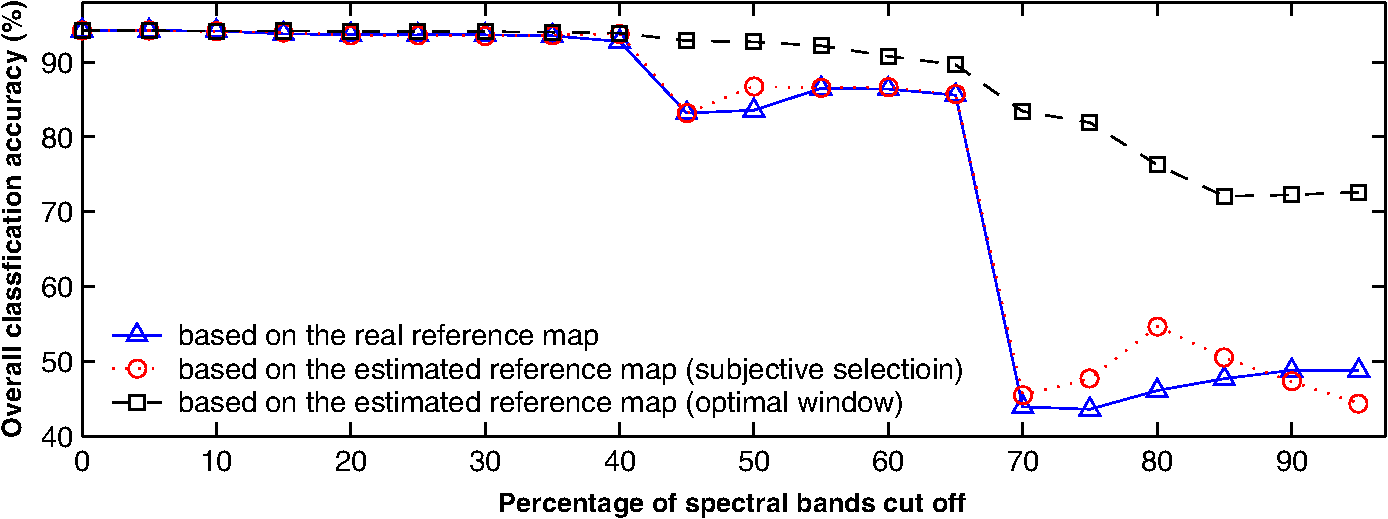
The local maxima are found by repeating the steps 2 and 3 until convergence is detected or a fixed number of iteration times is reached.23,27 To avoid the local maxima, a random-restart strategy is adopted, which runs an outer loop over the above gradient ascending in several wavelength regions. Every region can be obtained by dividing the whole spectrum evenly. Each outer loop chooses a random initial position in the region to start gradient ascending. If a new run of gradient ascending produces a better result than the stored one, it replaces the stored solution. After running out each region, the best final solution is found as the global submaxima. This strategy is simple but effective, which is evidenced by the experimental results shown in Sec. 4. 4.Experimental ResultsTo assess the proposed method, the public AVIRIS 92AV3C hyperspectral dataset is used. The dataset is illustrative of the problem of hyperspectral image analysis to determine land use. It can be downloaded from ftp://ftp.ecn.pur due.edu/biehl/MultiSpec/. Although the AVIRIS sensor collects nominally 224 bands of data (one per spectral band, ranging from 0.40 to 2.52 μm), four of these contain only zeros and so are discarded, leaving 220 bands in the 92AV3C dataset. Each image is of size pixels. The data cube was collected over a test site called Indian Pine in northwestern Indiana.2,28 4.1.Searching Spectral Window to Build a Reliable Reference MapIn the experiment, we first examine if the proposed scheme can find the optimal subset of bands to approximate the ground truth. We implement the algorithm introduced in Sec. 3 to search the optimal spectral window, with window widths varying from 20 to 50 bands, respectively. The number of samples for density estimation, i.e., , is 50, and the number of samples for entropy estimation, i.e., , is also 50. Selection of these two numbers is empirical in this research, and they are chosen to fit the specific application. Apparently, to estimate different probably density functions (PDFs), different and may be needed, and their values (i.e., the size of samples) should match the complexities of the approximated PDFs. Since we expect that the subset bands contain the most discriminatory information, they should achieve the highest classification accuracy of any other subsets. Hence, we compare the classification accuracies based on the bands within and outside the found spectral windows respectively. In the experiments, we chose support vector machines (SVMs)29,30 as the classifiers due to the higher dimensionality of input data. Also, previous works applying SVMs to hyperspectral data classification have shown competitive performance with the best available classification algorithms.28,31 However, other classification algorithms, including the unsupervised approaches, are also applicable since the band selection proposed in this research is independent of the classifier applied (actually, it can be categorized as a filtering method in the feature selection family). Figures 3(a) to 3(d) present the accuracy results under window widths of 20, 30, 40, and 50 bands, respectively. The solid lines denote the classification accuracy achieved by the found spectral window, and the star points are the classification results based on the other 200 random sampled spectral windows. The dashed lines stand for the means of the classification results from the 200 random sampled windows. The positions of the sampled spectral windows are decided by random numbers generated by the machine. The bands in these spectral windows are contiguous (see Fig. 5). The number of sampling is initially chosen as 200, which is in favor of the narrow window-width, such as 10 bands. In the case of wide window-width, such as 30, 40, or 50 bands, several repeats of sampling will happen, but this will not affect our comparison. It is seen that the accuracies based on the found spectral windows are indeed on the top of the results of all 200 random sampled windows, which justified the effectiveness of the searching algorithm. In other words, maximizing MI can indeed lead to finding of a good estimation of ground truth (i.e., the ideal classification result). Fig. 3Comparison of classification accuracy: - stands for the accuracy achieved by the found spectral windows, and ∗ the 200 random sampled windows as a function of the random sample sequence order; the widths of spectral window are (a) 20 bands, (b) 30 bands, (c) 40 bands, and (d) 50 bands.  Therefore in this experiment, the window-width is chosen as 35 bands. The above experiments are mainly used for justification of the algorithm. In practical applications, we can use MI value as the indication of the classification accuracy and do not need to implement the real classification test. The window-width is an application-related parameter. How to choose this parameter is crucial to this method. Basically, we can set the window-width by two approaches. The first one is by a priori knowledge. For example, if the classes to be categorized are known, we can refer to the existing spectral libraries and measure the widths of the absorption valleys (i.e., a particular spectrum where the light is absorbed by the constituent atoms or molecules; usually these spectra are like valleys in a spectral curve). Then, the size (in wavelength) of the spectral window can be chosen as the maximum of the absorption valleys’ widths. The second way is by a validation test using the training data. Figure 4(a) shows the maximal MI found by different window-widths. It is seen that when is set between 30 and 40 bands, a higher MI value is found. Therefore in this experiment, the window-width is chosen as 35 bands. Figure 4(b) illustrates the accuracy change with respect to the positions of spectral windows. In this case, the starting band number of this spectral window is band no. 14. It should be noted that the above experiments are mainly used for justification of the algorithm. In practical applications, we can use MI value as an indication of the classification accuracy and do not need to implement the real classification test. We also verified the proposed method by visual comparison. In Fig. 5, we illustrate the spectral window found by the proposed method, together with three other random sampled spectral windows (to help visual observation, all hyperspectral images shown in this paper are transformed using a suitable false color palette). To facilitate this comparison, the width of the spectral window is set up as 10 bands. Figures 5(a) to 5(c) illustrate spectral bands corresponding to three 10-bands width random sampled windows. Figure 5(d) displays 10 band images corresponding to the spectral window found by the searching algorithm. Comparing these spectral images with the accompanied reference map in Fig. 5(e), it can be seen that the images found by the proposed method contain relatively more discriminatory information than other random sampled bands. In Fig. 5(d), we can see that the inherent scale varies across the bands and can roughly distinguish the outline of the reference map, whereas in the bands of Figs. 5(a) to 5(c), this becomes less clear or impossible (for example, the third random sampled window that is unfortunately located in the atmospheric water absorption area). The visual comparison is consistent with the numerical analysis in Fig. 3. Fig. 5Visual comparison of three random sampled spectral window with the optimal spectral window; window-width is 10 bands; (a) random sample window 1, (b) random sample window 2, (c) random sample window 3, (d) optimal window, and (e) the reference map.  Through the above accuracy comparison and visual observation, it is verified that the proposed algorithm can find a spectral window to maximize the classification accuracy. Based on this spectral window, we are able to construct the estimated reference map by averaging the bands within the spectral window, such as in Eq. (6). If a spectral window works well for the classification, it gives a good indication to show that the characteristics of these bands (e.g., the clustering or separability of pixels’ values) have good capability to predict the class label. This can give information similar (but in different coding) to the one that the ground truth can provide. So a spectral window that works well for classification will also be good to build a reference map. Meanwhile, because the pixel values of a band can be considered as another kind of coding of ground truth, the bands within the spectral window can be regarded as a series of weaker reference maps. The proposed method makes these bands positively correlated (see the window constraint), with higher classification accuracy (see MI evaluation and the searching strategy); averaging them can provide a better estimation of reference map by reducing noise and uncertainty. This is the simplest approach to build the reference map by taking advantage of the proposed method. After constructing the reference map, band selection can be carried out, which is described as follows. 4.2.Results on Band SelectionThe main objective of band selection is to remove redundant spectral bands without degrading the classification accuracy too much. The experiment was designed to assess the change of classification accuracy as spectral bands are progressively removed according to the ranked MI values. To compare with the previous research,28,32,33 we use a subscene comprising of four classes: corn-notill, soybeans-notill, soybeans-min, and grass/trees. Figure 6 shows the results for the three cases, where the MI was calculated with respect to the reference map accompanied with the dataset (the solid curve marked with triangle), the subjective estimated reference map (the dotted curve marked with circle) (note that this map is estimated by visual inspection from domain expert), and the optimally constructed reference map using the approach introduced in Sec. 3 (the dashed curve marked with rectangle), respectively. Data points in the figure are at 5% increments corresponding to removal of 11 bands at each step. The results depicted in Fig. 6 show that in this particular application scenario,
Fig. 7Individual mean classification accuracies on the four different classes: (a) corn-notill, (b) grass/trees, (c) soybeans-min, (d) soybeans-notill.  The results summarized in the above 2 showed another improvement was achieved by the proposed method: monotonic performance degradation. This is an expected result and means that the ranking order for bands-cutting is more consistent with their contribution to the classification accuracy. In contrast, the performance curves of the other benchmarked methods showed no such result. Finally, the accuracy degradation of the proposed method is slower than other methods, indicating a better robust performance for bands-cutting. To justify the proposed method furthermore, we carried out an experiment based on a high-resolution hyperspectral dataset, i.e., Pavia University scene of ROSIS sensor (by courtesy of Prof. Paolo Gamba from the Telecommunications and Remote Sensing Laboratory, Pavia University, Italy34). The number of spectral bands is 103, with image size of pixels. The spatial resolution is as high as 1.3 m per pixel, in contrast to the 20 m of the AVIRIS 92AV3C dataset. The dataset is also accompanied with a ground-truth map, which categorized the whole picture as nine types of materials, such as asphalt, meadows, gravel, trees, painted metal sheets, bare soil, bitumen, self-blocking bricks, and shadows. Figure 8 shows four examples of spectral bands for Pavia University scene and its ground truth. Following the similar approach to process AVIRIS 92AV3C dataset, we also tested our method on the Pavia University scene dataset. Figure 9 shows the spectral bands in two spectral windows, where Fig. 9(a) contains the bands in the spectral window found by the proposed method and Fig. 9(b) contains the bands from a random spectral window. It can be seen clearly that the bands in Fig. 9(a) are more clear and contain more discriminatory information than those in Fig. 9(b). This result coincides with our previous observation on the AVIRIS 92AV3C dataset (see results in Fig. 5). Fig. 9Spectral bands in (a) the spectral window found by the proposed method and (b) a randomly sampled spectral window.  By using the newly constructed reference map, we also assessed the change of classification accuracy as spectral bands are progressively selected. Table 1 lists the classification accuracies using SVMs as classifiers and the band subsets are selected from 5 to 85 bands, respectively (see the first row of Table 1). The second row of Table 1 lists the classification results using the reference map estimated from the suboptimal spectral window found by the proposed method. The third row contains the results using a randomly selected spectral window, and the fourth row lists the results using the ground-truth survey. It can be seen from Table 1 that when only five bands are selected for classification, the proposed method obtained 63.02% accuracy, compared to 60.92% (using ground-truth map) and 59.15% (using a random spectral window) of the two benchmarked methods. When about half of the bands (45 bands) are selected, the proposed method achieved 86.18% classification accuracy, only 1.5% lower than that using all the 103 bands. The results showed that the majority of the discriminatory information has already been included during band selection and confirmed the effectiveness of the proposed method. Table 1Comparison of classification accuracy, Pavia University scene.
Regarding the above results in Figs. 6 and 7 and Table 1, an interesting question may arise: why the estimated reference map generated a better result than that using the reference map accompanied with the dataset. This may be explained by the completeness of ground-truth labeling and the accuracy of the underlying probability estimation. First, in 92AV3C dataset, the ground truth is designated into 16 classes and they are not all mutually exclusive.34,35 But PDF requires that states of a random variable are mutually exclusive. In this case, using the data in the ground-truth map to estimate the reference map’s PDF may produce significant errors (mismatch of the PDF’s definition). On the other hand, using the proposed method to estimate PDFs may avoid this problem because different real values are used to label different classes and they are mutually exclusive. Second, the accompanied reference map actually only labeled about half of the ground truth, i.e., the 16 classes of vegetations. The other half of pixels, e.g., highway, rail track, etc., are all categorized as background, presumably, because they correspond to uninteresting regions or were too difficult to label. This may put a strong argument to adopt the estimated reference map in the MI calculation because the estimated reference map differentiates different classes by different pixels’ value and all pixels can be fully utilized. Third, in the accompanied reference map, each class is labeled by an integer. For example, in AVIRIS 92AV3C, 16 classes of vegetations are labeled by 16 integers from 1 to 16, and the background is labeled by 0. Consequently, the estimated probability density will distribute in the integer domain. On the other hand, the estimated reference map is obtained by averaging several real spectral images, and the classes are differentiated by the real numbers characterized by their particular reflectance values. Since the MI is used to measure the utility of each band that was valued at the spectral response, the probability distribution estimated from the real reflectance values will match the MI calculation more than that using the artificially labeled values. 5.ConclusionsWe have described a band-selection method for hyperspectral image analysis without relying on a prespecified reference map. In our method, the reference map is constructed by averaging the bands within an optimal spectral window, which is automatically found by gradient ascending algorithm. Since the estimated reference map is more suitable to the calculation of MI, the proposed method outperformed that using the accompanied reference map. Using the AVIRIS dataset, up to 55% of bands could be cut off without significant loss of classification accuracy. Meanwhile, its performance is much robust to accuracy degradation. The method should be useful for cases where the ground truth is difficult to obtain. Future work is carried out to develop a theoretical framework for the MI-based discrete transform and to investigate an adaptive algorithm for setting the spectral window’s width. AcknowledgmentsThe authors would like to thank the associate editor and the anonymous reviewers for their constructive suggestions and, particularly, for the “Pavia University scene” dataset provided by anonymous reviewers. The first author is currently supported by National Natural Science Foundation of China (No. 61375011), Natural Science Foundation of Zhejiang Province (No. LY13F030015, No. LQ13F050010), Scientific Research Foundation for the Returned Overseas Chinese (State Education Ministry, China), and partly by a 973 Project (No. 2012CB821204). Part of the research presented in this paper was carried out at the University of Southampton and was funded by British DTC and the General Dynamics. ReferencesD. Landgrebe,
“Hyperspectral image data analysis,”
IEEE Signal Process. Mag., 19
(1), 17
–28
(2002). http://dx.doi.org/10.1109/79.974718 ISPRE6 1053-5888 Google Scholar
D. Landgrebe,
“On information extraction principles for hyperspectral data: a white paper,”
(1997) http://dynamo.ecn.purdue.edu/landgreb/whitepaper.pdf Google Scholar
G. ShawD. Manolakis,
“Signal processing for hyperspectral image exploitation,”
IEEE Signal Process. Mag., 19
(1), 12
–16
(2002). http://dx.doi.org/10.1109/79.974715 ISPRE6 1053-5888 Google Scholar
D. ManolakisG. Shaw,
“Detection algorithms for hyperspectral imaging applications,”
IEEE Signal Process. Mag., 19
(1), 29
–43
(2002). http://dx.doi.org/10.1109/79.974724 ISPRE6 1053-5888 Google Scholar
D. Steinet al.,
“Anomaly detection from hyperspectral imagery,”
IEEE Signal Process. Mag., 19
(1), 58
–69
(2002). http://dx.doi.org/10.1109/79.974730 ISPRE6 1053-5888 Google Scholar
G. Hughes,
“On the mean accuracy of statistical pattern recognizers,”
IEEE Trans. Inf. Theory, 14
(1), 55
–63
(1968). http://dx.doi.org/10.1109/TIT.1968.1054102 IETTAW 0018-9448 Google Scholar
G. PetrieP. HeaslerT. Warner,
“Optimal band selection strategies for hyperspectral data sets,”
in Proc. of IEEE Int. Geoscience and Remote Sensing Symp.,
1582
–1584
(1998). Google Scholar
S. SerpicoL. Bruzzone,
“A new search algorithm for feature selection in hyperspectral remote sensing images,”
IEEE Trans. Geosci. Remote Sens., 39
(7), 1360
–1367
(2001). http://dx.doi.org/10.1109/36.934069 IGRSD2 0196-2892 Google Scholar
P. GrovesP. Bajcsy,
“Methodology for hyperspectral band and classification model selection,”
in IEEE Workshop on Advances in Techniques for Analysis of Remotely Sensed Data,
120
–128
(2003). Google Scholar
C.-I. Changet al.,
“A joint band prioritization and band-decorrelation approach to band selection for hyperspectral image classification,”
IEEE Trans. Geosci. Remote Sens., 37
(6), 2631
–2641
(1999). http://dx.doi.org/10.1109/36.803411 IGRSD2 0196-2892 Google Scholar
M. Velez-ReyesL. Jimenez,
“Subset selection analysis for the reduction of hyperspectral imagery,”
in Proc. of IEEE Int. Geoscience and Remote Sensing Symp.,
1577
–1581
(1998). Google Scholar
P. BajcsyP. Groves,
“Methodology for hyperspectral band selection,”
Photogramm. Eng. Remote Sens. J., 70
(7), 793
–802
(2004). http://dx.doi.org/10.14358/PERS.70.7.793 PGMEA9 0099-1112 Google Scholar
B. Guoet al.,
“Band selection for hyperspectral image classification using mutual information,”
IEEE Geosci. Remote Sens. Lett., 3
(4), 522
–526
(2006). http://dx.doi.org/10.1109/LGRS.2006.878240 IGRSBY 1545-598X Google Scholar
B. Guoet al.,
“Fast separability-based feature selection method for high-dimensional remotely-sensed image classification,”
Pattern Recognit., 41
(5), 1670
–1679
(2008). http://dx.doi.org/10.1016/j.patcog.2007.11.007 PTNRA8 0031-3203 Google Scholar
J. Price,
“Spectral band selection for visible-near infrared remote sensing: spectral-spatial resolution tradeoffs,”
IEEE Trans. Geosci. Remote Sens., 35
(5), 1277
–1285
(1997). http://dx.doi.org/10.1109/36.628794 IGRSD2 0196-2892 Google Scholar
N. Keshava,
“Best bands selection for detection in hyperspectral processing,”
in Proc. of IEEE Int. Conf. on Acoustics, Speech and Signal Processing,
3149
–3152
(2001). Google Scholar
D. Qian,
“Band selection and its impact on target detection and classification in hyperspectral image analysis,”
in IEEE Workshop on Advances in Techniques for Analysis of Remotely Sensed Data,
374
–377
(2003). Google Scholar
S. KaewpijitJ. L. MoigneT. El-Ghazawi,
“Automatic reduction of hyperspectral imagery using wavelet spectral analysis,”
IEEE Trans. Geosci. Remote Sens., 41
(4), 863
–871
(2003). http://dx.doi.org/10.1109/TGRS.2003.810712 IGRSD2 0196-2892 Google Scholar
C. ConeseaF. Masellia,
“Selection of optimum bands from TM scenes through mutual information analysis,”
ISPRS J. Photogramm. Remote Sens., 48
(3), 2
–11
(1993). http://dx.doi.org/10.1016/0924-2716(93)90059-V IRSEE9 0924-2716 Google Scholar
B. Aiazziet al.,
“Information-theoretic assessment of multi-dimensional signals,”
Signal Process., 85
(5), 903
–916
(2005). http://dx.doi.org/10.1016/j.sigpro.2004.11.025 SPRODR 0165-1684 Google Scholar
Q. TongB. ZhangL. Zheng, Hyperspectral Remote Sensing—Principles, Techniques, and Applications, Higher Education Press, Beijing, China
(2006). Google Scholar
P. ViolaW. Wells,
“Alignment by maximization of mutual information,”
in Proc. of 5th Int. Conf. on Computer Vision,
16
–23
(1995). Google Scholar
J. PluimJ. MaintzM. Viergever,
“Mutual-information-based registration of medical images: a survey,”
IEEE Trans. Med. Imaging, 22
(8), 986
–1004
(2003). http://dx.doi.org/10.1109/TMI.2003.815867 ITMID4 0278-0062 Google Scholar
K. Torkkola,
“Feature extraction by non-parametric mutual information maximization,”
J. Mach. Learn. Res., 3
(Mar), 1415
–1438
(2003). 1532-4435 Google Scholar
N. KwakC.-H. Choi,
“Input feature selection by mutual information based on parzen window,”
IEEE Trans. Pattern Anal. Mach. Intell., 24
(12), 1667
–1671
(2002). http://dx.doi.org/10.1109/TPAMI.2002.1114861 ITPIDJ 0162-8828 Google Scholar
W. M. Wells IIIet al.,
“Multi-modal volume registration by maximization of mutual information,”
Med. Image Anal., 1
(1), 35
–51
(1996). http://dx.doi.org/10.1016/S1361-8415(01)80004-9 MIAECY 1361-8415 Google Scholar
J. GualtieriR. Cromp,
“Support vector machines for hyperspectral remote sensing classification,”
Proc. SPIE, 3584 221
–132
(1998). http://dx.doi.org/10.1117/12.339824 Google Scholar
B. E. BoserI. M. GuyonV. N. Vapnik,
“A training algorithm for optimal margin classifiers,”
in Proc. of the Fifth Annual Workshop on Computational Learning Theory,
144
–152
(1992). Google Scholar
C. Burges,
“A tutorial on support vector machines for pattern recognition,”
Knowl. Discov. Data Min., 2
(2), 121
–167
(1998). http://dx.doi.org/10.1023/A:1009715923555 1384-5810 Google Scholar
F. MelganiL. Bruzzone,
“Classification of hyperspectral remote sensing images with support vector machines,”
IEEE Trans. Geosci. Remote Sens., 42
(8), 1778
–1790
(2004). http://dx.doi.org/10.1109/TGRS.2004.831865 IGRSD2 0196-2892 Google Scholar
C. A. Shahet al.,
“Some recent results on hyperspectral image classification,”
in Proc. of IEEE Workshop on Advances in Techniques for Analysis of Remotely Sensed Data,
346
–353
(2003). Google Scholar
B. Guoet al.,
“Adaptive band selection for hyperspectral image fusion using mutual information,”
630
–637 Philadelphia, Pennsylvania
(2005). Google Scholar
P. Gamba,
“Hyperspectral dataset: Pavia University scene,”
http://www.ehu.es/ccwintco/index.php/Hyperspectral_Remote_Sensing_Scenes Google Scholar
D. Landgrebe,
“Electrical and computational engineering, University of Purdue,”
http://dynamo.ecn.purdue.edu/landgreb/ Google Scholar
BiographyBaofeng Guo received his BEng degree in electronic engineering and his MEng degree in signal processing from Xidian University in 1995 and 1998, and his PhD degree in signal processing from the Chinese Academy of Sciences, Beijing, in 2001. From 2002 to 2004, he was a research assistant at the University of Bristol. From 2004 to 2009, he was a research fellow in the University of Southampton, United Kingdom. Since 2009, he has been with the School of Automation, Hangzhou Dianzi University, China. Robert I. Damper received his MSc degree in biophysics and his PhD degree in electrical engineering from the University of London, London, United Kingdom, in 1973 and 1979, and his diploma in electrical engineering from Imperial College, London. He is a chartered engineer and a fellow of the U.K. Institution of Engineering and Technology, a chartered physicist, and a fellow of the U.K. Institute of Physics. Steve R. Gunn received his BEng degree (first class honors) in electronic engineering and his PhD degree in computer vision from the University of Southampton, Southampton, United Kingdom, in 1992 and 1996, respectively. He is currently a professor in the School of Electronics and Computer Science, University of Southampton. James D. B. Nelson received his BSc degree in mathematics and his PhD degree for his work on the application of Riesz bases to signal theory from Anglia Polytechnic University, United Kingdom He has held research posts at the Cranfield University, United Kingdom (three years) and the University of Southampton, Southampton, United Kingdom (two years), and is currently a research associate at the University of Cambridge, Cambridge, United Kingdom. |