Influence of surface height variance on distribution of ground control points

Sudniran Phetcharat; Masahiko Nagai; Taravudh Tipdecho

doi:10.1117/1.JRS.8.083684

29 January 2014 Influence of surface height variance on distribution of ground control points

Sudniran Phetcharat, Masahiko Nagai, Taravudh Tipdecho

Author Affiliations +

Journal of Applied Remote Sensing, Vol. 8, Issue 1, 083684 (January 2014). https://doi.org/10.1117/1.JRS.8.083684

Abstract

The process of geometric correction of a satellite image requires a network of ground control points (GCPs), the density of which depends on the accuracy required. In this study, an approach to determine the distribution of the GCPs was developed based on dividing the surface terrain into zones of low- and high-height variances. Comparative statistics were investigated to summarize the optimum number and distribution of the GCPs. For a uniform arrangement of 10 GCPs, the accuracy using root mean square error was 7.19 m. This accuracy was improved to 6.13 m following the inclusion of just two additional GCPs in the zone of high-surface height variance. Thus, the transformation using the polynomial model and a set of GCPs, for which the surface variance in height was considered, resulted in greater accuracy than using the conventional uniformly distributed method. In addition, the time required for the trial-and-error selection of the locations of the GCPs was reduced. Our results suggest that a method that considers the variance in height of the surface terrain could be applied to various types of images such as satellite or aerial photography.

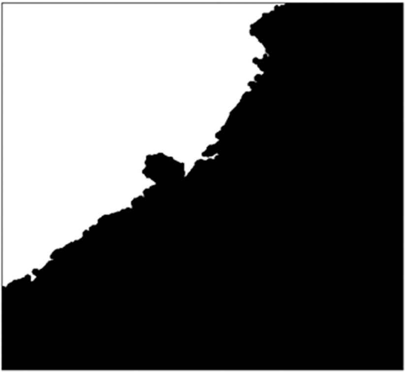
1. Introduction

Aerial photographs and satellite images are fundamental sources of data used for the analysis in geographic information systems, remote sensing, and mapping. The image acquisition process depends on the type of sensor used. Geometric distortion of the images from current pushbroom satellites, such as SPOT, ASTER, and Quickbird, is derived from two principal sources: inaccurate modeling of the charge-coupled device sensor geometry and small movements of the instrument platform during image acquisition.¹ High-resolution satellite images are prone to geometric distortion and thus, geometric correction is desirable.² The primary distortions have both internal and external sources. The former are the distortions inherent within a system that can be adjusted based on the characteristics of the sensor, e.g., lens distortion, which can be compensated for using the colinearity equation. The latter are the errors introduced from sources such as the Earth’s curvature and changes in atmospheric conditions, the reflective properties of light, and surface topography. These external sources distort the image directly, causing positions within the image to be inconsistent with those on the ground. Variations in elevation and surface roughness cause a particular type of distortion known as perspective distortion, which normally happens when using a short focal length.

In some cases, images used in satellite data analysis have no accompanying information regarding the sensor model of the satellite and thus, they may require adjustment using other appropriate models. Different methods for the transformation of one coordinate system to another have been proposed,³ e.g., the Helmert transformation, affine transformation, pseudo-affine transformation, projective transformation, second-order conformal transformation, and polynomial transformation. Of these, the polynomial model is simple and easy to use. Historically, polynomial models are among those empirical models used most frequently for fitting functions.⁴ The distortion is predominantly low frequency and therefore, it can be modeled using a low-order polynomial. Polynomials offer many advantages such as simple form, moderate flexibility of shapes, well-known and understood properties, and ease of use computationally. This model transforms three-dimensional (3-D) object coordinates to image coordinates and converts the data from 3D to two-dimensional (2-D). This transformation requires the use of ground control points (GCPs), which may be obtained using integrated information from ground surveys, photogrammetry, or GPS data comprising $x$ , $y$ , and $z$ coordinates. Rizos and Satirapod⁵ stated that the differential GPS technique generally provides an accuracy of better than 3 m in the horizontal component at twice the distance root mean square error (RMSE) (at approximately 95% confidence level). The results of the transformation are the coefficients of the polynomial equation.

Generally, GCPs for geometric correction are distributed uniformly throughout the entire image using a square grid.⁶ This approach is suitable for the calculation and determination of the GCP positions, but it does not account for onsite topography. The number of GCPs should be higher in mountainous areas or in areas with high variance of surface height. However, obtaining GCPs by field survey or other methods can be costly and time consuming; therefore, the optimization of the GCP network is desirable. The GCP locations should have high-spatial frequency and well-defined positions such as at river crossings and road junctions.⁷ Elevation is one of the three important variables needed to determine the coefficients of the 3-D polynomial equation and the positions of the GCPs. The GCPs should be located to sample the 3-D content of the data, i.e., a greater number of samples in regions of high height variation. Wang et al. stated that the spatial distribution of GCPs may affect the accuracy and quality of image correction.⁸ This study aims to determine the optimum number of GCPs required for each type of surface by classifying the level of height variance based on the standard deviation (SD) of the elevation distribution.

2. Study Area and GCP Availability

The study area is located in Chiang Mai and Lampoon, which are northern provinces of Thailand, approximately 600 km from Bangkok. This area has a variety of topographic characteristics including both flat areas and highly complex surfaces. The coordinates of the upper left and lower right corners of the target area are 98.83040° E, 18.7702° N and 99.02550° E, 18.5918° N, respectively, encompassing an area of approximately $406 {km}^{2}$ . The observed surface variance in height, based on a digital elevation model (DEM), is highly diverse, causing high values of SD and difference in elevation (the highest – the lowest), which are 69 and 643 m, respectively. Areas with high variance in height (mountainous terrain) accounted for $\sim 35 %$ of the area, mainly to the northwest; and the remaining 65% in eastern and southern parts of the image was areas with low variance in height (urban). Figure 1 shows an image of the landscape of this area acquired from Worldview-1 (Level 1B) on February 23, 2008. Level 1B data are radiometric-corrected, sensor-corrected, and band-aligned, providing imagery as seen from the spacecraft without any further correction of terrain distortion. Worldview-1 operates at an altitude of 496 km with a resolution of 50 cm in the panchromatic band at nadir. The specified geolocation accuracy of the instrument is less than 4.0 m CE90 (Circular Error of 90%) without GCPs in a 2-D image.⁹

Fig. 1

Study area in Chiang Mai and Lampoon, Thailand.

There are 78 GCP points with 3-D coordinates and accuracy of 0.2 m available for the image, which are provided by the Land Development Department of Thailand; however, only 68 GCP points were used in this study as independent check points (ICPs). The ICPs are those points that have been used in the RMSE process for checking the transformed image. A static and kinematic GPS survey was used to acquire the positions of the GCPs. All GCPs including the ICPs are shown in Fig. 2.

Fig. 2

All GCPs and ICPs across the digital elevation model (DEM).

3. Three-Dimensional Polynomial Model

Using GCPs to determine the coefficients, polynomial modeling is applied to generate a new surface model with enhanced accuracy, both in terms of shape and position of the image. Stability analysis of the polynomial differential equations is a central topic in nonlinear dynamics and control, which in recent years has undergone major algorithmic developments following advances in optimization theory.¹⁰ The transformation model creates a new geocoded image space, in which interpolated pixel values will be placed later during resampling. The procedure requires that the polynomial equations to be fitted to the GCPs using least squares criteria to model the geometrical distortion in the image domain independently of its source. The degree of the polynomial may be chosen based on the desired accuracy and the number of GCPs available. In general, polynomial equations used for modifying images are typically second or third order. The independent variables in the equation are $X_{n}$ , $Y_{n}$ , and $Z_{n}$ . The dependent variables are the row and column positions of the pixel ( $r_{p}$ and $c_{p}$ ).

For matching the point of the GCP chip on the ground and the associated point on the distorted image, the surrounding observation has been used. The coordinate functions are as shown below:

Eq. (1)

r_{p} = p_{v} (X_{n}, Y_{n}, Z_{n})

Eq. (2)

c_{p} = p_{h} (X_{n}, Y_{n}, Z_{n}),

where

r_{p}

is the position of the pixel in the row that corresponds to the column of the pixel in the distorted satellite image,

c_{p}

is the position of the pixel in the column that corresponds to the row of the pixel in the distorted satellite image, and

X

,

Y

,

Z

, and

n

are the ground coordinates that correspond to the east and north positions, elevation, and local position number, respectively.

Function $p_{v} (X_{n}, Y_{n}, Z_{n})$ and $p_{h} (X_{n}, Y_{n}, Z_{n})$ , as a second-order polynomial, can be generated from Eqs. (1) and (2) as follows:

Eq. (3)

r_{p} = a_{0} + a_{1} X_{n} + a_{2} Y_{n} + a_{3} Z_{n} + a_{4} X_{n} Y_{n} + a_{5} X_{n} Z_{n} + a_{6} Y_{n} Z_{n} + a_{7} X_{n}^{2} + a_{8} Y_{n}^{2} + a_{9} Z_{n}^{2} .

Eq. (4)

c_{p} = b_{0} + b_{1} X_{n} + b_{2} Y_{n} + b_{3} Z_{n} + b_{4} X_{n} Y_{n} + b_{5} X_{n} Z_{n} + b_{6} Y_{n} Z_{n} + b_{7} X_{n}^{2} + b_{8} Y_{n}^{2} + b_{9} Z_{n}^{2} .

Generally, polynomial transformations with terms up to the first order can model rotation, scale, and translation and are computationally economical. As additional terms are added, more complex warping can be achieved. $a_{j}$ and $b_{j}$ $(j = 0, 1, \dots, 9)$ are coefficients that are unknown but can be calculated using the least squares method from the error $E$ of all data $n$ deviating from the function $p (X_{n}, Y_{n}, Z_{n})$ as follows:

Eq. (5)

E = \sum_{i = 1}^{n} {[r_{p} - (a_{0} + a_{1} X_{i} + a_{2} Y_{i} + \dots + a_{9} Z_{i}^{2})]}^{2} .

Then, the minimum error can be found by differentiating $E$ with respect to the coefficient and setting the result to zero; thus, the following 10 subequations are produced:

Eq. (6)

\frac{\partial E}{\partial a_{0}} = 0, \frac{\partial E}{\partial a_{1}} = 0, \frac{\partial E}{\partial a_{2}} = 0, \dots, \frac{\partial E}{\partial a_{9}} = 0 .

The results of these equations will be in the form of a matrix with the following equation:

Eq. (7)

[\begin{matrix} n & \sum_{i = 1}^{n} X_{i} & \sum_{i = 1}^{n} Y_{i} & \dots & \sum_{i = 1}^{n} Z_{i}^{2} \\ \sum_{i = 1}^{n} X_{i} & \sum_{i = 1}^{n} X_{i}^{2} & \sum_{i = 1}^{n} X_{i} Y_{i} & \dots & \sum_{i = 1}^{n} X_{i} Z_{i}^{2} \\ \sum_{i = 1}^{n} Y_{i} & \sum_{i = 1}^{n} X_{i} Y_{i} & \sum_{i = 1}^{n} Y_{i}^{2} & \dots & \sum_{i = 1}^{n} Y_{i} Z_{i}^{2} \\ ⋮ & ⋮ & ⋮ & \dots & ⋮ \\ \sum_{i = 1}^{n} Z_{i}^{2} & \sum_{i = 1}^{n} X_{i} Z_{i}^{2} & \sum_{i = 1}^{n} Y_{i} Z_{i}^{2} & ⋱ & \sum_{i = 1}^{n} Z_{i}^{4} \end{matrix}] [\begin{matrix} a_{0} \\ a_{1} \\ a_{2} \\ ⋮ \\ a_{9} \end{matrix}] [\begin{matrix} \sum_{i = 1}^{n} r_{p} \\ \sum_{i = 1}^{n} X_{i} r_{p} \\ \begin{matrix} \sum_{i = 1}^{n} Y_{i} r_{p} \\ ⋮ \\ \sum_{i = 1}^{n} Z_{i}^{2} r_{p} \end{matrix} \end{matrix}] .

On the left side of this equation, a symmetric matrix “A” represents the known values square matrix ( $10 \times 10$ ), and matrix “B” denotes the coefficients matrix ( $10 \times 1$ ). On the right side, matrix “C” represents the known value matrix ( $10 \times 1$ ). Therefore, the multiplication of both sides of Eq. (7) with inverse matrix A provides the coefficients $a_{0}, a_{1}, a_{2}, \dots, a_{9}$ .

4. Surface Variance in Height Classification Method

Bayer et al.¹¹ stated that the synthetic aperture radar images reveal radiometric image distortions that are caused by terrain undulations, because the 3-D nature of the surface is ignored and GCPs are distributed uniformly here. We account for this and increase the sampling density depending on local variations of elevation. Here, two zones were chosen for these data; however, this may not be optimal. One method to allow for this would be to partition the image into several regions based on height variation and to have different GCP densities in the different regions. Many histogram-based approaches identify a threshold for the binarization of an image by approximating a histogram as two distribution functions.¹²^–¹⁴ Wu et al. proposed procedures for change-point detection (threshold selection) by determining the maximum distance from a line L to a cumulative histogram, where line L connects the first and last points of the cumulative histogram (Fig. 3).¹⁵ The main advantage of this method is being able to use the height to find a change-point of the surface variance in height. It is also appropriate for a large number of data points.

Fig. 3

Change-point detection and selection of a threshold using a cumulative histogram.

In Fig. 3, the straight line L connecting $(x_{1}, y_{1})$ and $(x_{N}, y_{N})$ is a cumulative “equalized” histogram. Histogram equalization modifies the pixel values in such a way that the intensity histogram of the resulting height becomes uniform.¹⁶ The maximum distance to L provides a baseline for dividing the cumulative histogram into two parts. The point $(x_{T}, y_{T})$ , representing the maximum distance to L, is the change-point to be used as the threshold. Line L can be obtained from the following equation:

Eq. (8)

\frac{(y - y_{1})}{(x - x_{1})} = \frac{(y - y_{N})}{(x - x_{N})} .

Assume that the obtained line equation is as shown below:

Eq. (9)

a x + b y + c = 0 .

The distance from $(x_{i}, y_{i})$ to L is expressed as follows:

Eq. (10)

\frac{| a x_{i} + b y_{i} + c |}{\sqrt{a^{2} + b^{2}}} .

Compare the distances of all $(X_{i}, Y_{i})$ points, where $2 \leq i \leq N - 1$ , to L and set $T = \arg \max_{i = 2}^{N - 1}$ $D [(X_{i}, Y_{i}), L]$ . Thus, the selected threshold is $X_{T}$ .¹⁵

4.1.

Change-Point Determination Using the Elevation Distribution

The classification of surface height variance, based on elevation data, was conducted using grid-based DEM data. The DEM data with resolution of 30 m were downloaded from the Global DEM and operated jointly by NASA and the Japan Ministry of the Economy. These data were then used to create a graph of the frequency distribution. The change-point was determined using the cumulative distribution curve.

Figure 4 shows the elevation on the $x$ -axis, the number of pixels in each elevation interval on the left side $y$ -axis, and the cumulative percentage at each elevation interval on the right side $y$ -axis. Based on this graph, the change-point for elevation was determined to be 308 m.

Fig. 4

Elevation histogram and cumulative distribution.

4.2.

Change-Point Determination Using the SD Distribution

The SDs represent the variance in height. Each SD is calculated using the eight pixels that surround a pixel of interested from a $3 \times 3$ elevation matrix. Therefore, the same calculation can be used to determine all the SDs for the entire image. The method proposed by Wu et al.¹⁵ was also used to determine the change-point based on the SD histogram.

Figure 5 shows a SD histogram with the SDs plotted on the $x$ -axis, the number of pixels in each SD interval shown on the left side $y$ -axis, and the cumulative percentage of the SDs presented on the right side $y$ -axis. Based on this graph, the SD change-point was determined to be 3.

Fig. 5

Standard deviation (SD) histogram and cumulative distribution.

4.3.

Classification and Zoning

After the change-points were determined, both the elevation frequency distribution and the SD frequency distribution were used to classify the surface into zones. The classification was conducted by designating those areas with elevation $> 308 m$ or $SD > 3$ as zones with high variance of height and necessarily, those areas with elevation $< 308 m$ or $SD < 3$ were classified as zones with low variance of height.

The final zoning of the area using Global Mapper software is shown in Fig. 6. It can be seen clearly that the area is divided into two zones following the change-point detection process. The white part represents the zone of high variance in height, and the black part represents the zone of low variance in height.

Fig. 6

Two zones divided through variance in height classification.

5. Number of GCPs and GCP Allocation

5.1.

Number of GCPs for Each Zone

The model used for geometric correction and for identifying the numbers and positions of the GCPs in this study was a second-order 3-D polynomial. As shown above, there are 10 variables in the form of coefficients in the polynomial: $a_{0}$ to $a_{9}$ . The number of GCPs required for this model is 10 per image. The image was classified into two zones using the zoning method described above, and the 10 points were distributed between these two zones. The number of GCPs assigned to each zone was determined after consideration of the zones size and degree of height variance.

The percentages of the total area (measured from the image) assigned to the two zones without consideration of the degree of variance in height were 35% (0.35) and 65% (0.65), respectively. The trial weights for the degree of variance in height ranged from 40% to 70% for four cases.

Table 1 shows five scenarios for the case being studied. In the first scenario, the 10 GCPs were distributed uniformly throughout the entire area. The proportional areas of the two zones were the same for all cases. For example, the calculation for Case II was conducted with the area of high variance in height assigned an influence of 40% and a proportional area of 35% (fixed). Accordingly, the area of low variance in height had an influence of 60% and a proportional area of 65% (also fixed). Based on this information, the number of GCPs to be distributed into each zone was determined to be 4 and 6 for the low and high variances in height zones, respectively. The results for all scenarios are shown in Table 1.

Table 1

Trial percentages of influence of the variance in height and number of GCPs for each zone.

Cases	High-variance in height		Low-variance in height
Cases	% Influence	GCPs - $N$	% Influence	GCPs - $N$
I	35	3.5	65	6.5
II	40	4	60	6
III	50	5	50	5
IV	60	6	40	4
V	69	7	30	3

5.2.

GCP Allocation

In general, GCPs are used in uniform distribution patterns. Points should first be placed on the four corners of the image to control the accuracy of regional mapping.¹⁷ Then, the other GCPs should be distributed uniformly within each zone. In this study, the selection of the locations of the GCPs was conducted manually. The locations of the GCPs for the five trial cases, based on the numbers of GCPs presented in Table 1, are shown in Fig. 7.

Fig. 7

GCP allocation for each trial case: (a) I—uniformly distributed, (b) II, (c) III, (d) IV, and (e) V.

Figure 7(a) shows Case I, in which the GCPs were allocated using the uniform distribution method. Four GCPs were placed at the corners to control the boundaries of the study area. The fifth GCP was placed at the center of the area, and the remaining five GCPs were spaced equally around the fifth point, resulting in a pentagon shape. The variance in height was not considered in this case.

For Cases II to V presented in Figs. 7(b) to 7(e), the GCP allocation based on a uniform distribution was conducted as follows:

1. Ten assumed points were defined within the study area, corresponding to the coefficients in the polynomial ( $a_{0}$ to $a_{9}$ ), and each point is circled to show clearly the definition applied in each trial case.
2. First, four GCPs were allocated near the four corners of the image.
3. The other priority GCPs should be allocated to the corners of each zone.
4. Then, an available GCP is selected as close as possible to the center of each assumed point.
5. The remaining GCPs should be allocated in other areas within the same zone for an equidistant coverage.

6. Results and Evaluation of Accuracy

The evaluation of accuracy was conducted by cross-checking the GCP positions on the transformed image in 2-D $(X_{est}, Y_{est})$ against the actual locations at the same positions on the ground in 2-D $(X_{act}, Y_{act})$ . The ground coordinates for the transformed image can be expressed by reversing Eqs. (3) and (4), because the polynomial transformation can be reversed from object coordinates to image coordinates, or vice versa. The accuracy of the transformation was determined using the RMSE with all the remaining 68 ICPs scattered throughout the image. The equation used in this calculation was as follows:¹⁸

Eq. (11)

RMSE = \sqrt{\frac{{[\sum_{i = 1}^{n} {(X_{act} - X_{est})}^{2}] + [\sum_{i = 1}^{n} {(Y_{act} - Y_{est})}^{2}]}}{n}},

where

n

is the number of all remaining ICPs,

X_{act}

and

Y_{act}

are the actual control points’

X

and

Y

coordinates, and

X_{est}

and

Y_{est}

are the estimated control points’

X

and

Y

coordinates.

Table 2 shows the RMSEs results when the GCP distribution was selected by varying the numbers and locations of the GCPs. It can be concluded that Case I is the best case because it shows the lowest average RMSE. This is probably because Case I applied a uniform distribution, which is a popular method for allocating GCPs. Furthermore, the variance in height of the surface in this case was ignored. The other cases that resulted in an increasing RMSE after the GCP positions were moved from the area of low variance in height to the area with high variance in height.

Table 2

RMSEs for the ICPs.

Case	RMSE
	ICP- $X$ (m)			ICP- $Y$ (m)			Average $X - Y$ (m)
	Total	High	Low	Total	High	Low	Total	High	Low
Case I	2.33	3.74	0.97	6.80	11.31	1.85	7.19	11.91	2.09
Case II	2.64	3.56	1.71	6.92	10.44	3.40	9.69	11.03	4.45
Case III	2.85	3.38	2.57	7.33	9.44	6.11	9.80	10.03	6.62
Case IV	23.77	4.95	42.58	69.96	15.87	124.04	73.88	16.62	131.14
Case V	52.27	7.87	62.33	169.95	24.23	202.74	177.81	25.48	212.10

To compare the 68 points in the transformed image, 68 ICPs were used and the evaluated direction of error, both in the $x$ - and $y$ -axes, is presented in Fig. 8. It was necessary to enlarge the scale by a factor of 100 to show clearly the direction of error. Furthermore, Fig. 8 shows that there were still errors in the upper-left corner of the map of error, corresponding to the zone of high variance in height.

Fig. 8

Map of error, Case II.

To confirm that the surface variance in height influenced the accuracy of the geometric correction of the image, a number of GCPs were removed or added to the zone of high variance in height and low variance in height; the different number of GCPs used per trial was two points. The results from this validation are presented in Tables 3 and 4.

Table 3

RMSEs of GCPs removed and added in high-variance zone.

Number of GCPs in high variance zone (added)	Number of all GCPs	RMSE			Remark
Number of GCPs in high variance zone (added)	Number of all GCPs	High	Low	All ICPs	Remark
1 ( $- 2$ )	8	37.71	16.17	26.08	Uniformly distributed
3 (0)	10	11.91	2.09	7.19
5 ( $+ 2$ )	12	10.39	2.88	6.31
7 ( $+ 4$ )	14	11.19	2.80	6.58
9 ( $+ 6$ )	16	11.13	2.72	6.21
11 ( $+ 8$ )	18	12.05	2.78	6.39

Note: Remark: (−) indicates GCPs removed, and (+) represents GCPs added.

Table 4

RMSEs of GCPs removed and added in low-variance zone.

Number of GCPs in low variance zone (added)	Number of all GCPs	RMSE			Remark
Number of GCPs in low variance zone (added)	Number of all GCPs	High	Low	All ICPs	Remark
5 ( $- 2$ )	8	24.74	17.45	20.05	Uniformly distributed
7 (0)	10	11.91	2.09	7.19
9 ( $+ 2$ )	12	12.12	2.06	7.36
11 ( $+ 4$ )	14	12.43	2.80	7.49
13 ( $+ 6$ )	16	12.32	2.18	7.68
15 ( $+ 8$ )	18	12.52	2.36	7.84

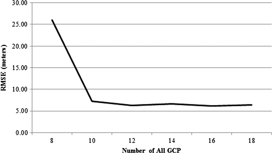
Note: Remark: (−) indicates GCPs removed, and (+) represents GCPs added.

By increasing and decreasing the number of GCPs in the zone of high variance in height, it was determined that the number of GCPs cannot be reduced below 10, as shown clearly in Fig. 9 by the rapid increase in RMSE when the number of GCPs was reduced from 10 to 8. The RMSE decreased by about 12% following the increase in the number of GCPs from 10 to 12. No significant improvement in accuracy can be observed by increasing the number of GCPs beyond 12.

Fig. 9

Effect of removing/adding GCPs in high-variance zone.

Increasing or decreasing the number of GCPs in the low variance in height zone resulted in the same trend found in the high variance in height zone; however, the results did not show any significant improvement in accuracy following an increase in the number of GCPs beyond 10 (Fig. 10).

Fig. 10

Effect of removing/adding GCPs in low-variance zone.

7. Conclusions

In this study, an image of mountainous terrain of the Chiang-Mai area acquired by Worldview I, a global DEM, and 78 ground truth points with an accuracy of 0.2 m were used to evaluate the accuracy of distortion correction using a polynomial model. Using the turning point from the elevation and SD histogram, the terrain was divided into two regions: low variance in height and high variance in height. This study determined the RMSE of the GCPs’ coordinates and demonstrated that the distribution of the GCPs affects the accuracy. In particular, it was shown that a uniform distribution of GCPs was the best arrangement. The effect of increasing or decreasing the number of GCPs in the high/low variance in height zones was investigated for the case of uniform distribution. The results conclude that a suitable minimum number of GCPs was 10 and that the accuracy was improvable by including just two additional GCPs in the zone of high variance in height, but that increase in the number of GCPs in the zone of low variance in height offered no significant improvement in accuracy.

The results of this study could be applied to aerial photographs or satellite images as guidance for identifying the optimum numbers and locations of GCPs for each zone of variance in height, especially for study areas with a variety of surface types. Through this approach, researchers could save time on the trial-and-error selection of locations for GCPs.

References

1.

F. Ayoubet al., “Influence of camera distortions on satellite image registration and change detection applications,” in IEEE International Geoscience and Remote Sensing Symposium, 1072 –1075 (2008). Google Scholar

2.

F. ArifM. AkbarA. M. Wu, “Geometric correction of high resolution satellite imagery and its residual analysis,” in International Conference on Advances in Space Technologies, 162 –166 (2006). Google Scholar

3.

F. H. MoffittE.M. Mikhail, Photogrammetry, 648 3rd ed.Harper & Row, New York (1980). Google Scholar

4.

C. CroarkinP. Tobias, “NIST/SEMATECH e-handbook of statistical methods,” (2013) http://www.itl.nist.gov/div898/handbook October ). 2013). Google Scholar

5.

C. RizosC. Satirapod, “Differential GPS-how good is it now?,” Meas. Map, 15 28 –30 (2001). Google Scholar

6.

J. ZhangB. Cheng, “Distribution optimization of ground control points in remote sensing image geometric rectification based on cluster analysis,” Proc. SPIE, 7497 749707 (2009). http://dx.doi.org/10.1117/12.833671 PSISDG 0277-786X Google Scholar

7.

J. HuangJ. Wang, “The selection of GCPs of remote sensing image correction [C],” in Environmental Remote Sensing Symposium Academic, 738 –742 (20042013). http://www.isprs.org/proceedings/XXXV/congress/comm4/papers/446.pdf Google Scholar

8.

J. Wanget al., “Effect of the sampling design of ground control points on the geometric correction of remotely sensed imagery,” Int. J. Appl. Earth Obs. Geoinf., 18 (1), 91 –100 (2012). http://dx.doi.org/10.1016/j.jag.2012.01.001 0303-2434 Google Scholar

9.

( (2013) http://www.digitalglobe.com/resources/satellite-information October ). 2013). Google Scholar

10.

A. A. AhmadiP. A. Pablo, “Stability of polynomial differential equations: complexity and converse Lyapunov questions,” IEEE Trans. Autom. Control, (2012). IETAA9 0018-9286 Google Scholar

11.

T. BayerR. WinterG. Schreier, “Terrain influences in SAR backscatter and attempts to their correction,” IEEE Trans. Geosci. Remote Sens., 29 (3), 451 –462 (1991). http://dx.doi.org/10.1109/36.79436 IGRSD2 0196-2892 Google Scholar

12.

S. BoukharoubaJ. M. RebordaoP. L. Wendel, “An amplitude segmentation method based on the distribution function of an image,” Comput. Vision Graph. Image Process., 29 (1), 47 –59 (1985). http://dx.doi.org/10.1016/S0734-189X(85)90150-1 1753-8955 Google Scholar

13.

M. I. Sezan, “A peak detection algorithm and its application to histogram-based image data reduction,” Comput. Vision Graph. Image Process., 49 (1), 36 –51 (1990). http://dx.doi.org/10.1016/0734-189X(90)90161-N CVGPDB 0734-189X Google Scholar

14.

D. M. Tsai, “A fast thresholding selection procedure for multimodal and unimodal histograms,” Pattern Recogn. Lett., 16 (6), 653 –666 (1995). http://dx.doi.org/10.1016/0167-8655(95)80011-H PRLEDG 0167-8655 Google Scholar

15.

Q. Z. WuH. Y. ChengB. S. Jeng, “Motion detection via change-point detection for cumulative histograms of ratio images,” Pattern Recogn. Lett., 26 (5), 555 –563 (2005). http://dx.doi.org/10.1016/j.patrec.2004.09.010 PRLEDG 0167-8655 Google Scholar

16.

J. H. HanS. YangB. U. Lee, “A novel 3-D color histogram equalization method with uniform 1-D gray scale histogram,” IEEE Trans. Image Process., 20 (2), 506 –512 (2011). http://dx.doi.org/10.1109/TIP.2010.2068555 IIPRE4 1057-7149 Google Scholar

17.

Z. Wangfeiet al., “The selection of ground control points in a remote sensing image correction based on weighted Voronoi diagram,” in IEEE Int. Conf. Information Technology and Computer Science, 326 –329 (2009). Google Scholar

18.

K. T. Chang, Introduction to Geographic Information Systems, 3rd ed.McGraw-Hill, New York (2006). Google Scholar

Biography

Sudniran Phetcharat is a PhD student of the Asian Institute of Technology, Thailand. He received the B.Eng. degree in transportation engineering from Suranaree University of Technology, Nakonrachasima, in 1997, and an M.Eng. degree in civil engineering from Kasetsart University, Bangkok, in 2001. He has been an assistant professor with the Civil Engineering Department, Srinakharinwirot University, College Station. His research interests include crumb rubber-modified asphalt, highway materials, GIS application in transportation, and house saving energy.

Masahiko Nagai is an associate director of the Geoinformatics Center and a visiting faculty in the Asian Institute of Technology (AIT) in Thailand. He received the Master of Science from AIT and the Doctoral of Engineering from the University of Tokyo, Japan. His research focuses on geoinformatics, mainly environmental monitoring, Earth observation data interoperability arrangement with ontological information for remote sensing and GIS, construction of 3-D modeling by integrating multiple sensors, as well as disaster management.

Taravudh Tipdecho is a research specialist I (adjunct faculty) at the Asian Institute of Technology (AIT) in Thailand. He received his BS and MS degrees from Chiangmai University, Thailand, and D Tech Sc. degree from AIT, Thailand. His research focuses on the acquisition methods for large scale geoinformation. In recent years, the research focus has been on information extraction from airborne laser-scanning data. These interests also include accuracy analysis, image understanding, and object modelling.

CC BY: © The Authors. Published by SPIE under a Creative Commons Attribution 4.0 Unported License. Distribution or reproduction of this work in whole or in part requires full attribution of the original publication, including its DOI.

Citation Download Citation

Sudniran Phetcharat, Masahiko Nagai, and Taravudh Tipdecho "Influence of surface height variance on distribution of ground control points," Journal of Applied Remote Sensing 8(1), 083684 (29 January 2014). https://doi.org/10.1117/1.JRS.8.083684

Published: 29 January 2014

Access the abstract

JOURNAL ARTICLE
13 PAGES

DOWNLOAD PAPER SAVE TO MY LIBRARY

GET CITATION

CITATIONS

Cited by 1 scholarly publication.

Explore citations on Lens.org

KEYWORDS

3D modeling

Distortion

Satellite imaging

Satellites

Earth observing sensors

Image processing

3D image processing

1.

Introduction

2.

Study Area and GCP Availability