Forest height estimation from mountain forest areas using general model–based decomposition for polarimetric interferometric synthetic aperture radar images

Nghia Pham Minh; Bin Zou; Hongjun Cai; Chengyi Wang

doi:10.1117/1.JRS.8.083676

18 February 2014 Forest height estimation from mountain forest areas using general model–based decomposition for polarimetric interferometric synthetic aperture radar images

Nghia Pham Minh, Bin Zou, Hongjun Cai, Chengyi Wang

Author Affiliations +

Journal of Applied Remote Sensing, Vol. 8, Issue 1, 083676 (February 2014). https://doi.org/10.1117/1.JRS.8.083676

Abstract

The estimation of forest parameters over mountain forest areas using polarimetric interferometric synthetic aperture radar (PolInSAR) images is one of the greatest interests in remote sensing applications. For mountain forest areas, scattering mechanisms are strongly affected by the ground topography variations. Most of the previous studies in modeling microwave backscattering signatures of forest area have been carried out over relatively flat areas. Therefore, a new algorithm for the forest height estimation from mountain forest areas using the general model–based decomposition (GMBD) for PolInSAR image is proposed. This algorithm enables the retrieval of not only the forest parameters, but also the magnitude associated with each mechanism. In addition, general double- and single-bounce scattering models are proposed to fit for the cross-polarization and off-diagonal term by separating their independent orientation angle, which remains unachieved in the previous model-based decompositions. The efficiency of the proposed approach is demonstrated with simulated data from PolSARProSim software and ALOS-PALSAR spaceborne PolInSAR datasets over the Kalimantan areas, Indonesia. Experimental results indicate that forest height could be effectively estimated by GMBD.

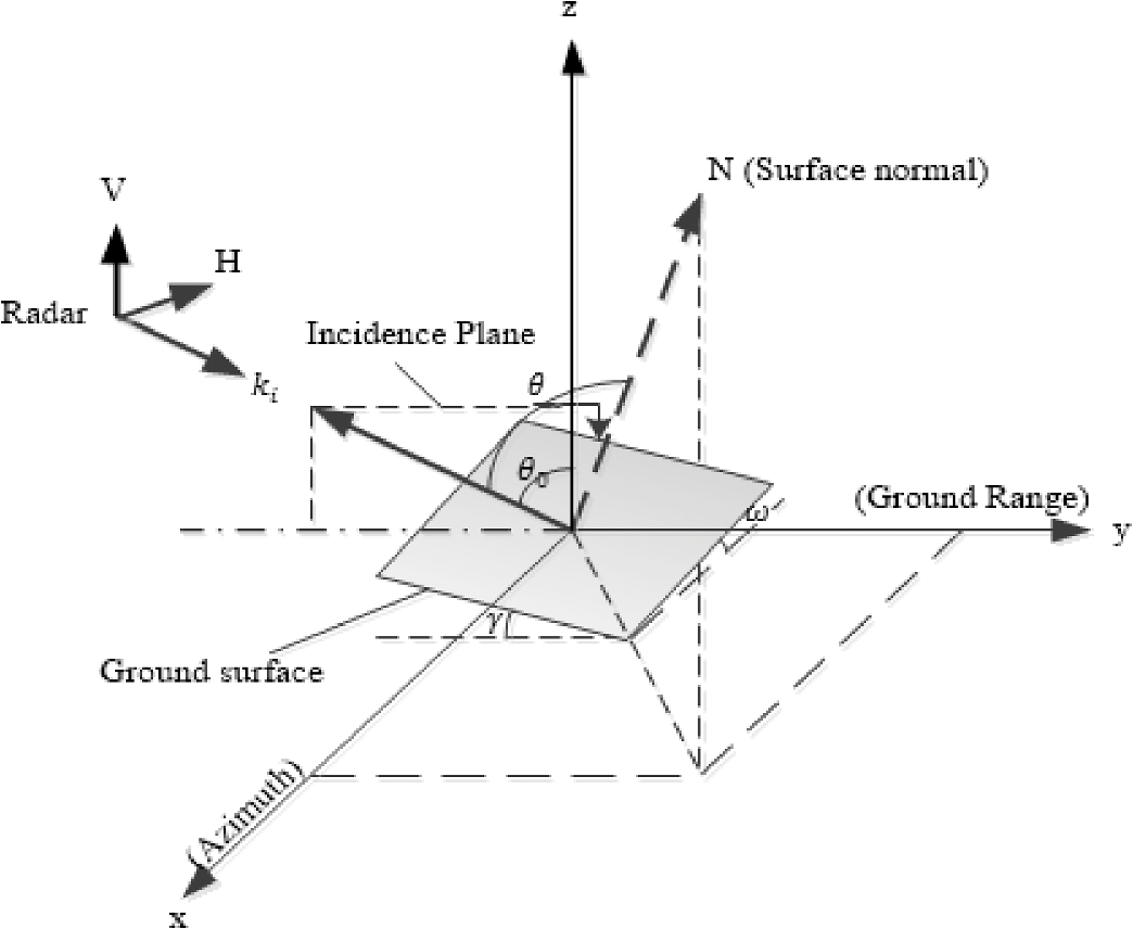
1. Introduction

Polarimetric interferometric synthetic aperture radar (PolInSAR) is a type of remote sensing technique that integrates the advantage of both polarimetric SAR and interferometric SAR. Therefore, retrieving parameters related to forest and monitoring the underlying soil surface have become one of the major applications in the field of active microwave remote sensing including SAR system. In the last 15 years, many techniques have been proposed for forest height estimation using single-baseline PolInSAR images, most of which can be broken up into two categories. The first group is based on the random volume over ground model as introduced by Cloude and Papathanassiou,¹ Yamaguchi et al.,² Garestier and Le Toan.³^–⁵ However, these methods tend to underestimate forest height due to attenuation of electromagnetic (EM) waves in the ground medium, and the accuracy of these methods becomes worse for dense forest areas due to the strong volume scattering component. The second major group is based on model-based decomposition technique for PolInSAR image as introduced by Ballester-Berman and Lopez-Sanchez⁶ and Neuman et al.⁷ The technique opened a new way for forest height estimation using the model-based decomposition technique. In this technique, they assumed that the volume contribution is a cloud of uniformly randomly distributed thin cylinders. However, natural forest canopy shows preferential orientation of the branches, smaller twigs, and leaves, which limits the applicability of the uniform randomly distributed model.⁸ So, this model is suitable for forest areas that assumes scattering reflection symmetry, but cannot be generalized for forest areas. One facet of this article is to provide an approach for canopy parameter estimation that is not constrained by these limits.

On the other hand, most previous studies were carried out over relatively flat areas. For mountain forest areas, scattered signals are strongly affected by the variations of the local incidence angle and the local orientation angle due to the local topographic slope. Results of VanZyl⁹ and Lin and Sarabandi¹⁰ indicated that the dominant scattering is changed drastically when the ground surface is tilted relative to the horizontal. In Ref. 11, Lee and Anisworth investigated the effect of ground topography on the coherency matrix and polarimetric target decomposition. However, in this method, the double- and single-bounce scatterings are still modeled with zero cross-polarization power. In order to overcome these limitations, general double- and single-bounce scattering models will be proposed by separating their independent orientation angles.

This article aims to present an accuracy improvement of forest height estimation over mountain forest that accounts for the effect of slope terrain on scattering mechanisms. In this article, we proposed a forest height estimation approach from mountain forest areas using general model–based decomposition (GMBD) technique for PolInSAR image. In this approach, we shall develop a general volume scattering model that can be characterized by two parameters: a degree of randomness and a mean orientation angle.⁸ After that, we will form a lookup database including reference volume scattering coherence matrices. The general volume scattering coherence matrix can be determined during the optimization procedure of the model inversion. The unknown parameters of forest can be obtained by using the nonlinear least square optimization method. Finally, the forest height is estimated by phase differencing between canopy phase and underlying ground phase. This algorithm enables the retrieval of not only the forest parameters above the tilted ground plane, but also the magnitude associated with each mechanism. In addition, the negative power can be avoided, and the proposed approach allows a more robust implementation and an unambiguous estimation of ground topography. Another advantage of the proposed algorithm is that it makes use of all the information provided by the interferometric coherence matrix, which remains unachieved in the previous model-based decompositions. Experimental results show that the accuracy of the forest height can be improved by the proposed approach.

The organization of this article is as follows. In Sec. 2, the forest scattering model for a sloping forest area is presented. The retrieval of forest height using GMBD algorithm is delivered in Sec. 3. The experimental results of the parametric inversion with simulated data are presented and discussed in Sec. 4. Summary and conclusions are drawn in Sec. 5.

2. General Scattering Model in Mountain Forest Areas for PolInSAR

2.1.

Polarimetric Interferometric Coherence Matrix in Mountain Forest Areas

A fully PolInSAR system is measured for each resolution cell in the scene from two slightly different look angles and two scattering matrices, [ $S_{1}$ ] and [ $S_{2}$ ]. For the case of reciprocal medium and monostatic backscattering, the individual polarimetric datasets may be expressed by means of the Pauli target vector¹²

Eq. (1)

{\vec{k}}_{P i} = \frac{1}{\sqrt{2}} {[S_{h h}^{i} + S_{v v}^{i} S_{h h}^{i} - S_{v v}^{i} 2 S_{h v}^{i}]}^{T},

where

{[]}^{T}

represents the vector transposition,

S_{p q}

(

p, q = {h, v}

) is the complex scattering coefficient, and

i = 1, 2

denotes the measurement at two ends of the baseline.

The basic radar observable in PolInSAR is a six-dimension complex matrix of a pixel in each resolution element in the scene, defined as shown in Eq. (2)

Eq. (2)

[T] = 〈 \vec{k} {\vec{k}}^{* T} 〉 = [\begin{matrix} T_{1} & Ω \\ Ω^{* T} & T_{2} \end{matrix}] with \vec{k} = [\begin{matrix} {\vec{k}}_{1} \\ {\vec{k}}_{2} \end{matrix}],

where

〈 \cdot 〉

denotes the ensemble average in the data processing, and * represents the complex conjugation.

[T_{1}]

and

[T_{2}]

are the conventional Hermitian polarimetric coherence matrices which describe the polarimetric properties for each individual image separately, whereas

[Ω]

is a non-Hermitian complex matrix which contains polarimetric and interferometric information.

For a tilted plane, the horizontal vector is no longer parallel to the surface; so, most of the polarization channels (HH, HV, VH, and VV) are affected by the tilted slope. The amount of slope-induced shift in the local orientation angle can be visualized as the rotation of the vertical–horizontal basis vector about the line-of-sight, so that the horizontal vector is again parallel to the surface. The local orientation angle is geometrically related to topographic slopes and radar look angles, and it is a function of the azimuth slope, the range slope, and the incidence angle of the flat terrain.¹¹ A schematic diagram depicting the radar image geometry is shown in Fig. 1. The local orientation angle change due to the azimuth slope effect can be expressed as

Eq. (3)

\tan ψ = \frac{\tan ω}{- \tan γ \cos θ_{0} + \sin θ_{0}},

where

γ

and

ω

are the local ground range and azimuth slopes, respectively. The angle

θ_{0}

is the incidence angle of the flat terrain.

Fig. 1

Schematic diagram of the imaging geometry for sloping ground surface.

For mountain terrain, the variation of the local incidence angle and the local orientation angle due to the local topography will lead to changes in the scattered signal.⁹ The polarimetric interferometric coherence matrix and coherence matrix in sloping terrain can be obtained by rotation of an orientation polarization angle.¹¹

Eq. (4)

[Ω (ψ)] = [R (ψ)] [Ω] {[R (ψ)]}^{* T} = [\begin{matrix} Ω_{11} (ψ) & Ω_{12} (ψ) & Ω_{13} (ψ) \\ Ω_{21} (ψ) & Ω_{22} (ψ) & Ω_{23} (ψ) \\ Ω_{31} (ψ) & Ω_{32} (ψ) & Ω_{33} (ψ) \end{matrix}],

with

Eq. (5)

[R (ψ)] = [\begin{matrix} 1 & 0 & 0 \\ 0 & \cos 2 ψ & \sin 2 ψ \\ 0 & - \sin 2 ψ & \cos 2 ψ \end{matrix}] and ψ = \frac{1}{4} \arctan {\frac{- 4 Re (〈 (S_{h h} - S_{v v}) S_{h v}^{*} 〉)}{- 〈 {| S_{h h} - S_{v v} |}^{2} 〉 + 4 〈 {| S_{h v} |}^{2} 〉}},

where

R (ψ)

is the unitary rotation matrix for the coherence matrix, and similar rotation transform was presented as in Ref. 11.

2.2.

Single-Bounce Contribution from Sloping Surface

In case of the flat surface, the single-bounce scattering model is presented by the first-order Bragg surface scatter, plate, and sphere, and triple-bounce scattering modeling is slightly rough surface scattering in which the cross-polarized component is negligible. The amplitude of the scattering coefficient does not change for both images, except the difference in the phase term. This phase term will have two contributions: the difference due to the complex scattering coefficient in the case of using different polarizations for master and slave images $φ_{h v} = φ_{h} - φ_{v}$ and the interferometric phase related to the position in the vertical coordinate $ϕ_{S}$ . Hence, the Pauli target vector of single-bounce contribution for both ends of the baseline is represented as

Eq. (6)

{\vec{k}}_{P 1} = \frac{1}{\sqrt{2}} [\begin{matrix} \cos α_{s} e^{j φ_{1}} \\ \sin α_{s} e^{j φ_{2}} \\ 0 \end{matrix}] and {\vec{k}}_{P 2} = \frac{1}{\sqrt{2}} [\begin{matrix} \cos α_{s} e^{j (φ_{1} + ϕ_{s})} \\ \sin α_{s} e^{j (φ_{1} + ϕ_{s})} \\ 0 \end{matrix}],

where the coefficients

φ_{1}

and

φ_{2}

account for wave propagation processing. We assume that these coefficients for master and slave images of the interferometric pair are the same. The real coefficient

α_{s} \leq π / 4

depends on dielectric constant and angle of incidence and is given as¹³

Eq. (7)

α_{s} = \arccos (\frac{| R {}_{H}+ R_{V} |}{\sqrt{{| R_{H} + R_{V} |}^{2} + {| R_{H} - R_{V} |}^{2}}}) .

The phase $ϕ_{s}$ denotes the interferometric phase for the direct scattering from surface. The coefficients $R_{H}$ and $R_{V}$ are the horizontal and vertical Fresnel reflection coefficients of the ground surface, respectively. In this case, the coherence matrix for the single-bounce contribution is expressed as

Eq. (8)

[T_{s}] = \frac{e^{j ϕ_{s}}}{2} [\begin{matrix} \cos^{2} α_{s} & \cos α_{s} \sin α_{s} e^{j φ_{s}} & 0 \\ \cos α_{s} \sin α_{s} e^{- j φ_{s}} & \sin^{2} α_{s} & 0 \\ 0 & 0 & 0 \end{matrix}],

with

Eq. (9)

φ_{s} = φ_{1} - φ_{2} .

For a rugged terrain surface, the presence of topographic variations induces the local incidence angle $θ$ to be a function of the local terrain slope

Eq. (10)

\cos θ = \frac{\tan γ \sin θ_{0} + \cos θ_{0}}{\sqrt{1 + \tan^{2} γ + \tan^{2} ω}},

where the angle

θ_{0}

is the incidence angle of the flat terrain. In addition, the presence of topography variations induces a local coordinate system in accordance with the tilted ground surface. In order to address the orientation of ground scattering, terms of the forest scattering model are superseded by the scattering from the slanted ground plane. In this case, the coherence matrix for the single-bounce contribution is obtained from the rotation of an orientation angle

χ

.

Eq. (11)

[T_{s} (χ)] = [R (χ)] [T_{s}] {[R (χ)]}^{* T} = \frac{e^{j ϕ_{s}}}{2} [\begin{matrix} 2 \cos^{2} α_{s} & 2 \cos α_{s} \sin α_{s} \cos 2 χ e^{j φ_{s}} & - 2 \cos α_{s} \sin α_{s} \sin 2 χ e^{j φ_{s}} \\ 2 \cos α_{s} \sin α_{s} \cos 2 χ e^{- j φ_{s}} & 2 \sin^{2} α_{s} \cos^{2} 2 χ & - \sin^{2} α_{s} \sin 4 χ \\ - 2 \cos α_{s} \sin α_{s} \sin 2 χ e^{- j φ_{s}} & - \sin^{2} α_{s} \sin 4 χ & 2 \sin^{2} α_{s} \sin^{2} 2 χ \end{matrix}] .

Slope also modifies the apparent alpha parameter $α_{s}$ for the surface backscatter. The range slope component will cause an increase (for slopes away from the radar) or decrease (for slopes toward the radar) in the apparent alpha parameter. In this article, we assume that the range slope is away from the radar.

2.3.

Double-Bounce Contribution from Sloping Surface

The double-bounce scattering component is modeled by scattering from the interaction between the ground and tree trunk or stem, where the reflector surface can be made of different dielectric materials. Hence, the Pauli target vector of double-bounce contribution for master and slave images can be expressed in the form

Eq. (12)

{\vec{k}}_{P 1} = \frac{1}{\sqrt{2}} [\begin{matrix} \cos α_{D} e^{j φ_{3}} \\ \sin α_{D} e^{j φ_{4}} \\ 0 \end{matrix}] and {\vec{k}}_{P 2} = \frac{1}{\sqrt{2}} [\begin{matrix} \cos α_{D} e^{j (φ_{3} + ϕ_{D})} \\ \sin α_{D} e^{j (φ_{4} + ϕ_{D})} \\ 0 \end{matrix}],

where

α_{D} \geq π / 4

depends on the angle of incidence and the two dielectric constants of the surface and reflector, which is represented as follows:

Eq. (13)

α_{D} = \arccos (\frac{| R_{GH} R_{TH} - R_{GV} R_{TV} |}{\sqrt{{| R_{GH} R_{TH} + R_{GV} R_{TV} |}^{2} + {| R_{GH} R_{TH} - R_{GV} R_{TV} |}^{2}}}) .

The coefficients $R_{GH}$ and $R_{GV}$ are the horizontal and vertical Fresnel reflection coefficients of the ground surface, respectively. Similarly, the vertical trunk surface has reflection coefficients $R_{TH}$ and $R_{TV}$ for horizontal and vertical polarizations, respectively. These coefficients are assumed to be equal for both ends of the baseline. Hence, the coherence matrix for the double-bounce contribution is given by

Eq. (14)

[T_{D}] = \frac{e^{j ϕ_{D}}}{2} [\begin{matrix} \cos^{2} α_{D} & \cos α_{D} \sin α_{D} e^{j φ_{D}} & 0 \\ \cos α_{D} \sin α_{D} e^{- j φ_{D}} & \sin^{2} α_{D} & 0 \\ 0 & 0 & 0 \end{matrix}],

with

Eq. (15)

φ_{D} = φ_{3} - φ_{4} .

In the double-bounce scattering component, the backscatter ray path no longer includes the two specular reflection mechanisms for two surfaces over sloping terrain surface. For this reason, the presence of slopes can attenuate the backscatter dihedral return and leave only the direct surface component. The slope tolerance of the double-bounce component depends on many factors such as the height of the vertical scatterer and radar wavelength. Instead of considering this phenomenon on a case-by-case basis, we prefer to model surface as some a priori unknown mixture of single- and double-bounce scattering mechanisms. Hence, the coherence matrix for the double bounce in mountain forest areas is obtained by the rotation of an orientation angle $η$ .

Eq. (16)

[T_{D} (η)] = [R (η)] [T_{D}] {[R (η)]}^{* T} = \frac{e^{j φ_{D}}}{2} [\begin{matrix} 2 \cos^{2} α_{D} & 2 \cos α_{D} \sin α_{D} \cos 2 η e^{j φ_{D}} & - 2 \cos α_{D} \sin α_{D} \sin 2 η e^{j φ_{D}} \\ 2 \cos α_{D} \sin α_{D} \cos 2 η e^{- j φ_{D}} & 2 \sin^{2} α_{D} \cos^{2} 2 η & - \sin^{2} α_{D} \sin 4 η \\ - 2 \cos α_{D} \sin α_{D} \sin 2 η e^{- j φ_{D}} & - \sin^{2} α_{D} \sin 4 η & 2 \sin^{2} α_{D} \sin^{2} 2 η \end{matrix}] .

For flat terrain surface, the surface and dihedral component are orthogonal.¹⁴ The orthogonal condition can be expressed as

Eq. (17)

α_{s} + α_{D} = \frac{π}{2} and φ_{D} - φ_{s} = \pm π .

Therefore, the orthogonal condition reduces $(α_{S}, α_{D})$ to $α$ and $(φ_{S}, φ_{D})$ to $φ$ in Eqs. (11) and (16). Therefore, two equations [Eqs. (11) and (16)] are written as

Eq. (18)

[T_{s} (κ)] = \frac{e^{j φ_{s}}}{2} [\begin{matrix} 2 \cos^{2} α & - 2 \cos α \sin α \cos 2 κ e^{j φ} & 2 \cos α \sin α \sin 2 κ e^{j φ} \\ - 2 \cos α \sin α \cos 2 κ e^{- j φ} & 2 \sin^{2} α \cos^{2} 2 κ & - \sin^{2} α \sin 4 κ \\ 2 \cos α \sin α \sin 2 κ e^{- j φ} & - \sin^{2} α \sin 4 κ & 2 \sin^{2} α \sin^{2} 2 κ \end{matrix}]

Eq. (19)

[T_{D} (η)] = \frac{e^{j φ_{D}}}{2} [\begin{matrix} 2 \sin^{2} α & 2 \cos α \sin α \cos 2 η e^{j φ} & - 2 \cos α \sin α \sin 2 η e^{j φ} \\ 2 \cos α \sin α \cos 2 η e^{- j φ} & 2 \cos^{2} α \cos^{2} 2 η & \cos^{2} α \sin 4 η \\ - 2 \cos α \sin α \sin 2 η e^{- j φ} & \cos^{2} α \sin 4 η & 2 \cos^{2} α \sin^{2} 2 η \end{matrix}] .

2.4.

General Volume Scattering Model

The volume scattering is direct diffuse scattering from the canopy layer of forest model. In mountain forest areas, volume scattering component is not much affected by the tilt of the ground surface because trees on a slope grow in alignment with gravity and sunlight. So, the scattering from the canopy layer of forest can be reasonably characterized by a cloud of randomly oriented infinitely thin cylinders.⁸^,¹⁵ In the theoretical modeling of volume scattering, a cloud of randomly oriented dipoles is implemented with a uniform probability function for the orientation angles. However, for forest areas where vertical structure seems to be rather dominant, the scattering from tree trunks and branches displays a nonuniform angle distribution. Therefore, we assume the volume scattering contribution with an $n$ ’th power cosine-squared distribution of orientation with probability density function as Ref. 16. The parameter $n$ ranges from zero to infinity. In practice, there is little difference between distributions with values of $n$ larger than about 20 or so. It can be shown that the standard deviation $σ$ can be evaluated in terms of $n$ , as in Ref. 8. The standard deviation $σ$ varies in a range between 0 and 0.91. It changes with the corresponding change in distribution function from delta to uniform distribution function for the vegetation orientation angles. Then, the volume scattering coherence matrix is expressed as

Eq. (20)

[T_{v} (\bar{θ}, σ)] = [T_{a}] + p (σ) [T_{b} (2 \bar{θ})] + q (σ) [T_{c} (4 \bar{θ})],

where

\bar{θ}

is the mean orientation angle of dipoles. The coefficients

p (σ)

and

q (σ)

are characterized by sixth-order polynomials, as in Ref. 8. The basic coherence matrices

[T_{a}], [T_{b}]

, and

[T_{c}]

are expressed as

Eq. (21)

[T_{a}] = \frac{1}{4} [\begin{matrix} 2 & 0 & 0 \\ 0 & 1 & 0 \\ 0 & 0 & 1 \end{matrix}] [T_{b}] = \frac{1}{4} [\begin{matrix} 0 & 2 \cos 2 \bar{θ} & 2 \sin 2 \bar{θ} \\ 2 \cos 2 \bar{θ} & 0 & 0 \\ 2 \sin 2 \bar{θ} & 0 & 0 \end{matrix}] [T_{c}] = \frac{1}{4} [\begin{matrix} 0 & 0 & 0 \\ 0 & \cos 4 \bar{θ} & \sin 4 \bar{θ} \\ 0 & \sin 4 \bar{θ} & - \cos 4 \bar{θ} \end{matrix}] .

3. Forest Height Extraction Based on GMBD

In this section, we propose the algorithm for the estimation of forest height in mountain forest areas using GMBD for PolInSAR image. For PolInSAR data, the polarimetric interferometric coherence matrix after rotation by orientation angle is expressed as follows:

Eq. (22)

[Ω (ψ)] = f_{s} e^{j ϕ_{s}} [T_{s} (χ)] + f_{D} e^{j ϕ_{D}} [T_{D} (η)] + f_{v} e^{j ϕ_{v}} [T_{v} (\bar{θ}, σ)] + [T_{remainder}],

where

f_{S}

,

f_{D}

, and

f_{v}

represent the scattering power coefficient of single bounce, double bounce, and volume scattering, respectively.

χ

and

η

are the rotation angles for single- and double-bounce scattering, respectively.

T_{remainder}

is the residual term which should be minimized after the decomposition. The Frobenius norm of remainder component can be used to determine the best fit parameter to express the measured polarimetric interferometric radar data. Therefore, the optimization criteria are

Eq. (23)

\min : {‖ T_{remainder} ‖}_{2} .

In this section, we first find the volume coherence matrix from Eq. (20). In forest area, the backscattering of an EM depends on the shape, size, and orientation of leaves, small branches, and tree trunk. Therefore, we will form the lookup database including the volume scattering mechanism models in Refs. 15 and 17 18.–19 as a reference volume scattering model. These models not only are suitable for geophysical media symmetry, but also satisfy the conditions for geophysical media asymmetry.

In this article, we suggest that each of the reference volume scattering coherence matrices in the lookup database can be used to determine the best-fit parameter to express the general volume scattering matrix. For each of the reference volume scattering coherence matrices in the lookup database, we implemented finding of the volume scattering, so that $[T_{v}^{i} (\bar{θ}, σ)]$ approximates to the reference volume scattering coherence matrix by varying the randomness $σ$ and mean orientation angle $\bar{θ}$ for the entire range.⁸ These parameter sets are equivalent to a best fit under condition that subtraction of general volume scattering coherence matrix and reference volume scattering matrix becomes zero. The optimal volume scattering model can be determined during the optimization procedure of this model. When the set of generalized volume scattering coherence matrices is determined based on the lookup database, we can obtain the set of canopy phase and the coefficient $f_{v}$ as follows:

Eq. (24)

f_{v}^{i} = | \frac{Ω_{33} (ϕ) - Ω_{22} (ϕ)}{T_{v (33)}^{i} - T_{v (22)}^{i}} |

Eq. (25)

φ_{v}^{i} = \arg {\frac{Ω_{33} (ϕ) - Ω_{22} (ϕ)}{T_{v (33)}^{i} - T_{v (22)}^{i}}},

where

i = 1, 2, \dots, N

;

N (N = 5)

denotes the total matrices in lookup database of reference volume scattering coherence matrices.

Ω_{m n} (ψ)

and

T_{v (m n)}^{i}

represent the element of the column

m

and the row

n

of the matrix

Ω (ϕ)

and

T_{v}^{i}

, respectively.

After subtracting the resulting volume component, Eq. (22) becomes

Eq. (26)

[Ω_{remainder}] = [Ω (ϕ)] - f_{v}^{i} e^{j φ_{v}^{i}} [T_{v}^{i} (\bar{θ}, σ)] = f_{s}^{i} e^{j φ_{s}^{i}} [T_{s}^{i} (κ)] + f_{D}^{i} e^{j φ_{D}^{i}} [T_{D}^{i} (η)] + [T_{remainder}^{i}] .

As can be seen, in matrix $[Ω_{remainder}]$ , there appear eight real unknowns ${f_{s}, f_{D}, ϕ_{s}, ϕ_{D}, α, φ, χ, η}$ , a matrix $[T_{remainder}^{i}]$ , and nine complex observables, since $Ω_{remainder (i, j)} \neq Ω_{remainder (j, i)}$ . This formulation leads to a determined nonlinear equation system. Therefore, to determine the rest of the unknown parameters ${f_{s}, f_{D}, ϕ_{s}, ϕ_{D}, α, φ, χ, η}$ and $[T_{remainder}^{i}]$ simultaneously, the nonlinear least square optimization method is implemented.²⁰ In order to improve the quality of this proposed method, the initial values for orientation angle of single bounce $κ$ and double bounce $η$ are all equal to $- \frac{π}{4}$ (Ref. 10). With each pair value ( $χ, η$ ), the parameters ${f_{s}, f_{D}, ϕ_{s}, ϕ_{D}, α, φ}$ are determined by employing an singular value decomposition of the $Ω_{remainder}$ . The parameter set ${f_{s}, f_{D}, ϕ_{s}, ϕ_{D}, α, φ, χ, η}$ in this step is determined from condition minimum of Frobenius norm of matrix ${[T_{remainder}]}_{i}$ . We show that the parameter set ${f_{s}, f_{D}, f_{v}, ϕ_{s}, ϕ_{D}, ϕ_{v}, α, φ, χ, η}$ is equivalent to a best fit under condition that the Frobenius norm of remainder matrix becomes zero, where the estimated parameters are perfectly matched to the observations. Finally, we repeat both the above steps for each pixel in the image. The algorithm is summarized in Fig. 2. When the optimal parameters are obtained from GMBD, we can extract the surface topography phase as in Eq. (27)

Eq. (27)

φ_{s} = \arg {Ω_{11} (ϕ) - \frac{{| A |}^{2}}{B^{*}}},

with

Eq. (28)

A = \frac{Ω_{12} (ϕ) \sin 2 κ + Ω_{13} (ϕ) \cos 2 κ}{\cos 2 η \sin 2 κ - \sin 2 η \cos 2 κ} and B = \frac{Ω_{22} (ϕ) \sin 4 κ + 2 Ω_{23} (ϕ) \cos^{2} 2 κ}{\cos^{2} 2 η \sin 4 κ - \sin 4 η \cos^{2} 2 κ} .

Fig. 2

General model–based decomposition (GMBD) algorithm for single pixel.

Based on the obtained optimization parameters from general decomposition approach, the forest height in mountain forest areas can be extracted by using the phase differencing in Eq. (29)

Eq. (29)

h_{v} = \frac{φ_{v} - φ_{s}}{k_{z}} = Δ φ \frac{λ}{4 π} \frac{R \sin θ}{B \cos (θ - δ)},

where

θ

is the mean angle of incidence,

R

is the distance between the radar and an observed point,

δ

is the baseline tilt angle,

B

is the baseline, and

λ

is the wavelength.

4. Experimental Results and Discussion

In this section, the effective evaluation of the proposed approach is addressed in terms of the retrieved forest height estimation and ground phase. For such a purpose, we have applied the proposed method to a dataset acquired from PolSARProSim software by William²¹ as well as spaceborne data acquired by the ALOS-PALSAR system.

4.1.

Simulated PolInSAR Data

First, the proposed approach has been evaluated by the simulated forest scenario and considering different slope terrains, which are generated with the PolSARProSim software. The simulated data are realized at 1.3 GHz, and the interferometer is operated at 10-m horizontal and 1-m vertical baseline. The stand height 18 m is located on a 18-deg ground azimuth and 6-deg ground range slope. The forest stand occupies a 0.82745 ha area, with a stand density of 360 stem/ha. Azimuth and slant range resolutions are 1.5 and 1.06 m, respectively. Figure 3(a) shows a red, green, blue (RGB) coding Pauli image of the forest scenario considered, and the red line indicates the transection analyzed in this article with $139 \times 129$ pixels. Figure 3(b) is a plot of the forest height estimation by using GMBD compared with the three-stage inversion and adaptive decomposition methods in the 124th row of azimuth transect line.¹

Fig. 3

Pauli image on RGB coding of simulated data (a) and histogram of the height results comparison (b).

Table 1 indicates that the proposed method is more accurate and has less error than the three-stage inversion and adaptive decomposition methods. The three-stage inversion is the most used coherence model for coherence optimization, and it requires multiple-parameter least square estimation, which is complex and often ill-conditioned. Besides, this method assumed the vertical structure, and minimum ground-to-volume scattering ratio needs to be lower than $- 10 dB$ to secure around 10% accuracy.¹ Otherwise, the forest height and extinction estimation by using three-stage inversion process is not reliable, and only the underlying ground topographic phase is reliable. Based on Fig. 3 and Table 1, we can say that the forest height and ground phase estimations by using GMBD are more accurate and reliable than that by using three-stage inversion process and adaptive decomposition.

Table 1

Forest height estimation for three approaches.

Parameters	True	Three-stage inversion	Adaptive decomposition	Proposed method
$h_{v}$ (m)	18	13.4619	14.2123	17.2751
$Φ_{0}$ (rad)	$- 0.148$	$- 0.1452$	$- 0.1350$	$- 0.1160$
Average error (m)	0	4.5381	3.7877	0.7294
RMSE (m)	0	2.4290	4.6987	5.2801

Changes in the scene parameters can be noticed by means of the proposed method. Table 2 shows the forest parameters estimation with difference slope terrains. The rest of the parameters remain unchanged. The interferometric phase is affected remarkably by both azimuth and ground ranges slopes. So, for the forest height estimation methods related with phase, it will be hard to obtain the right value.²² In the proposed method, the accuracy of interferometric phase is significantly improved by orientation compensation and by choosing the best-fit parameter for each scattering mechanism using the solving of the nonlinear least square optimization. From Table 2, we show that the local ground range slopes $γ$ from 0 to 30 deg and the local ground azimuth slope $ω$ all range from 0 to 45 deg. Table 2 shows that the forest height decreases when increasing azimuth slope. Especially, the forest height is less accurate at $(γ, ω) = (30 \deg, 45 \deg)$ , but the accuracy of it is relatively high, at 89.96%. Based on Table 2, we can say that the forest height and ground phase estimations by using GMBD are relatively accurate and reliable.

Table 2

Forest parameter estimation for difference slope terrains.

Parameters	True	$γ = 0 \deg$ $ω = 6 \deg$	$γ = 0 \deg$ $ω = 27 \deg$	$γ = 6 \deg$ $ω = 18 \deg$	$γ = 18 \deg$ $ω = 30 \deg$	$γ = 27 \deg$ $ω = 45 \deg$	$γ = 30 \deg$ $ω = 45 \deg$
$h_{v}$ (m)	18	17.2096	17.0145	17.2751	17.1461	16.8917	16.1935
$Φ_{0}$ (rad)	$- 0.148$	$- 0.1425$	$- 0.1371$	$- 0.1350$	$- 0.1022$	$- 0.1135$	$- 0.1131$
Average error (m)	0	0.7904	0.9855	0.7294	0.8539	1.1083	1.8065
RMSE (m)	0	5.0174	5.2545	5.2801	4.8822	4.9909	3.6979

4.2.

Spaceborne PolInSAR Data

Next, the effective evaluation of the proposed approach is addressed with spaceborne data. The dataset used in this section is acquired from an image pair of the Kalimantan region, Indonesia, by the ALOS-PALSAR system observed on March 12 and April 27, 2007, respectively. The baseline of the two observations is 330 m at the scene center, and the spatial resolution of the test data is $30 \times 10 m^{2}$ . They consisted of full polarized data at L-band with 21.5-deg angle of incidence and composed of $12,816 \times 1129 pixels$ . The optical image from Google Earth and the color image of the classical Pauli decomposition are shown in Figs. 4(a) and 4(b), respectively.

Fig. 4

L-band PALSAR data of Kalimantan region. (a) Optical image from Google Earth. (b) Pauli decomposition of test data.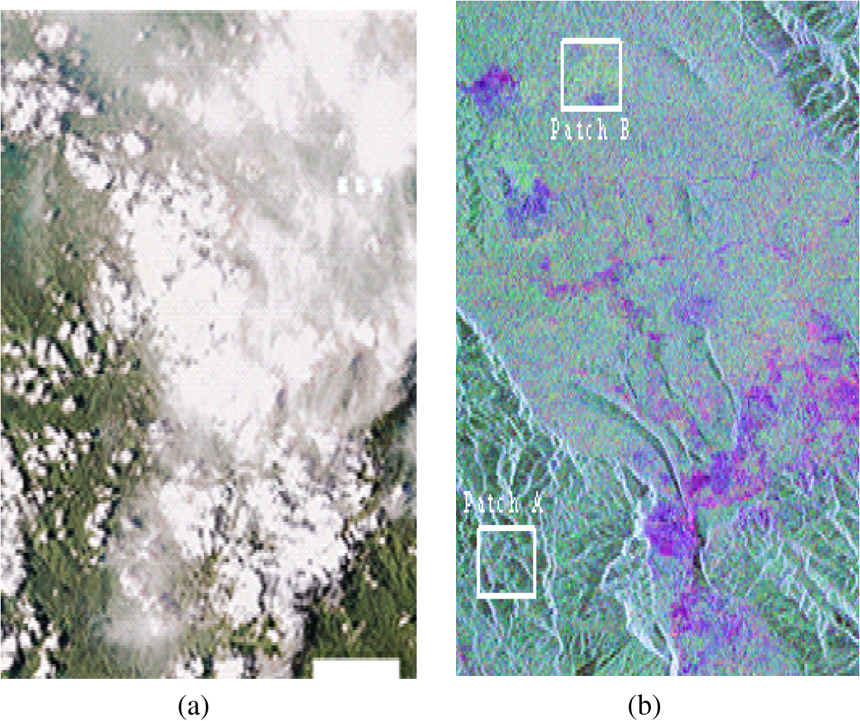

The Kalimantan area contains heterogeneous objects such as forest area, agricultural area (violet area), and mountains covered with trees. As analyzed by Papathanassiou and Cloude,²³ the presence of temporal correlation coefficient leads to a decrease of the amplitude of the interferometric coherence, but does not affect the position of the effective phase centers. Furthermore, the amplitude of the interferometric coherence of test site data (after co-registration image and filtering procedures) is almost greater than 0.6, and the forest height of the proposed method is estimated by using the difference phase method. Hence, in this section, we neglect the effect of the temporal decorrelation.

After co-registration of PolInSAR image, we select two regions of interest from Fig. 4(b) for further comparison including mountain forest area A with $375 \times 384$ and forest area B with $265 \times 481$ . Patch B contains mainly pure forest, whereas patch A includes mostly mountains covered with trees. Figure 5(a) is a plot of the forest height estimation of the proposed approach compared with adaptive model–based decomposition²⁴ with orientation angle compensation in patch A. For a fair comparison, all these methods are implemented on the polarimetric interferometric coherence matrix. This figure shows that the forest height of the proposed approach is located in a range from 16 to 24 m, whereas the forest height of the adaptive model–based decomposition method is located in a range from 3 to 23 m. The parameters of forest over two patches are calculated and shown in Table 3. This table indicates that the proposed approach is more accurate and less error prone than the adaptive model–based decomposition approach, even though the adaptive model–based decomposition was compensated by the rotation coherence matrix for the orientation effect. Orientation angle compensation can reduce these cross-polarization powers and better decomposition performance can be achieved. However, the estimated polarization orientation angle is a mixture among all the scattering mechanisms for a coherence matrix. So, this approach cannot always guarantee for cross-polar the single- and double-bounce scattering contributions back to zero. This is a possible reason that the canopy phase and underlying ground phase estimation ambiguities still appear, especially at the mountain forest areas. The results concerning the retrieval of the fraction fill canopy of trees $r_{h}$ are presented in Table 3. The fraction fill canopy of trees is determined as follows:

Eq. (30)

r_{h} = \frac{2.7 \ln {\bar{h}}_{v} - 0.1}{h_{v}} .

Fig. 5

Forest height estimation. (a) Histogram of the height results comparison, and (b) forest height estimation from the proposed algorithm.

Table 3

Parameter estimation for two approaches.

Parameter	Patch A		Patch B
Parameter	Adaptive	Proposed	Adaptive	Proposed
$h_{v}$ (m)	17.2845	19.3794	17.6490	19.3604
$r_{h}$	0.4394	0.4079	0.4335	0.4085
$Φ_{0}$ (rad)	$- 0.0180$	$- 0.0161$	0.0313	0.0302
RMSE ( $h_{v}$ ) (m)	9.2848	8.0722	5.3888	5.0172

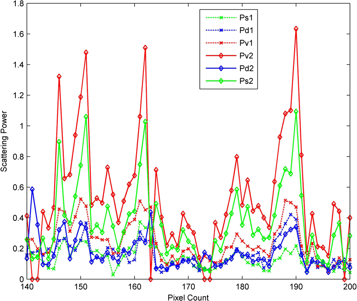
Figure 5(b) shows the estimated forest height by the proposed approach in mountain forest A. This figure shows that most of the peak differentials of the forest height are located approximately at 20 m. The forest height estimation at some pixels is overestimated by less than 25 m. The real effective tree height will be higher than these values, so we can say that the results are acceptable. Based on Fig. 5 and Table 3, we can say that the forest height estimation and the underlying ground topographic phase are reliable. Consequently, the proposed approach provides relative accuracy with small error and more accurate for vertical structural variations, especially at the sloping terrain.

To estimate the main forest parameters, the presented forest model in the alternate transmit model is used. The parameter inversion process consists of optimizing the error function and estimating the physical parameters $h_{v}$ , $r_{h}$ , $f_{v}$ , $ϕ_{v}$ , $\bar{θ}$ , $σ$ , $f_{d}$ , $α$ , $φ$ , $ϕ_{d}$ , $η$ , $f_{s}$ , $ϕ_{s}$ , and $χ$ . Figure 6 presents the parameter inversion performance in the 200th row of mountain forest A. The height sensitivity is given by the vertical wavenumber, which is about 0.16. This corresponds to $2 π$ height ambiguity of about 40 m. In the experiments, the graphs display the value and the standard deviation of estimated parameters. This figure indicates that the total forest height is around 20 m [Fig. 6(a)], the underlying topographic phase is around 0 rad [Fig. 6(d)], the mean orientation angle of volume scattering contribution is around 65 deg [Fig. 6(c)], and the degree of orientation randomness of volume scattering contribution is very low ( $σ \approx 0$ ) [Fig. 6(b)].

Fig. 6

Parameter estimation for mountain forest A ( $375 \times 384$ ). (a) Forest height, (b) degree of orientation randomness of volume scattering, (c) mean orientation angle of volume scattering, and (d) underlying topographic phase.

The rotation angle of single- and double-bounce scattering components estimated by GMBD approach over mountain forest A is shown in Fig. 7. In this figure, it is shown that the large rotation angle for single-bounce scattering contribution in these areas ( $χ \approx 40 \deg$ ) and the rotation angle for double-bounce angle for double-bounce contribution is around 23 deg. This is caused by the dominance of surface scattering contribution in the sloping terrain and the increasing of the cross-polarization and off-diagonal terms.

Fig. 7

Rotation angle maps derived in mountain forest A.

To evaluate the proposed decomposition further, the derived scattering power for the proposed approach and the adaptive model–based decomposition method without orientation compensation corresponding to mountain forest A are shown in Fig. 8. Evidently, the results of the adaptive model–based decomposition show that the double-bounce scattering contribution ( $P_{d 1}$ ) is too low, and the volume scattering ( $P_{v 1}$ ) is relatively high. In the proposed decomposition, the double-bounce scattering power ( $P_{d 2}$ ) is significantly enhanced. The power of the surface scattering component ( $P_{s 2}$ ) is remarkably increased.

Fig. 8

Comparison of scattering components for two methods.

The scattering power contributions of the three scattering components are calculated and are also compared in Table 4. For forest area B, which corresponds to a relatively flat area, the two methods show relatively equivalent results. In this area, the volume scattering is dominant and very high: 94.6% for the adaptive decomposition and 96.6% for the proposed method. For mountain forest area A, for the adaptive decomposition, although the volume scattering component is still dominant, the percentage of dominant $P_{v}$ is reduced to 75.99% while the percentage of dominant single- and double-bounce contributions $P_{s}$ and $P_{d}$ are increased to 11.04% and 12.97%, respectively. For the proposed decomposition, even though the dominant volume scattering is still maximal, the percentage of dominant $P_{v}$ is significantly decreased to 62.98%. Otherwise, the percentage of surface scattering component $P_{s}$ is significantly increased to 20.45%. The percentage of double bounce is relatively increased to 16.57%. The reason lies in that the scattering mechanisms in patch A is strongly affected by the topographic variations. In addition, the topographic variations introduce changes in the penetration depth of microwave into the forest. Thereby, the occurrences of the ground-trunk double-bounce scattering are not as many as those of single-bounce scattering directly from the trunks or branches. Therefore, the reduced volume scattering power mainly changes into the single-bounce scattering.

Table 4

Power of three scattering components (%) over two study areas.

Method	Mountain forest A			Forest B
Method	$P_{s}$	$P_{d}$	$P_{v}$	$P_{s}$	$P_{d}$	$P_{v}$
Adaptive	11.04	12.97	75.99	2.5	2.9	94.6
Proposed	54.19	16.57	29.24	1.2	2.2	96.6

Figure 9 corresponds to the amplitude of the three scattering mechanisms contributing to the $HH + VV$ [Fig. 9(a)] channel and $HH - VV$ [Fig. 9(b)] channel in the mountain forest area A. As shown, the amplitude of volume scattering contribution is dominant for all two channels, whereas the amplitude of surface scattering component is also remarkable for $HH + VV$ channel (as predicted by theories in Refs. 1 and 6). For $HH - VV$ channel, the amplitude of double-bounce scattering component is too high, but it is not dominant due to slope of terrain.

Fig. 9

Amplitude contributions of the three scattering mechanisms to (a) $HH + VV$ channel and (b) $HH - VV$ channel.

5. Conclusions

The underestimation of the forest height and the scattering mechanism ambiguities over sloping terrain in the model-based decomposition and the height estimation method was discussed. The GMBD scheme, which uses all polarimetric interferometric coherence matrix elements, has been proposed. All the model parameters and forest height can be adaptively obtained during the optimization procedure of the model inversion. In comparison to other methods, the proposed approach enables us to improve the estimation of forest height and ground topography over mountain forest area, as well as to retrieve additional parameters related to the degree of randomness, the main orientation of particles, the canopy layer depth, and power contribution of each scattering component. The GMBD approach is quite flexible and effective for analysis of more complex forest model over all types of terrains with PolInSAR images. Experimental results indicate that the forest parameters can be retrieved directly and more accurately using the proposed approach. In the future, further theoretical and experimental investigations will be done to improve the performance of the proposed approach.

Acknowledgments

This work was supported by National Natural Science Foundation of China under Grant No. 61271348 and National S&T Plans in Agriculture Area in the Twelfth Five-Year Period (No. 2011BAD08B02-03).

References

1.

S. R. CloudeK. P. Papathanassiou, “Three-stage inversion process for polarimetric SAR interferometric,” IEE Proc. Radar Sonar Navig., 150 (3), 125 –134 (2003). http://dx.doi.org/10.1049/ip-rsn:20030449 1350-2395 Google Scholar

2.

H. Yamadaet al., “Polarimetric SAR interferometry for forest analysis based on the ESPRIT algorithm,” IEICE Trans. Electron., 84 (12), 1917 –2014 (2001). IELEEJ 0916-8524 Google Scholar

3.

F. GarestierT. Le Toan, “Evaluation of forest modeling for forest height estimation using P-band PolInSAR data,” in Proc. BIOGEOSAR, (2007). Google Scholar

4.

F. GarestierT. Le Toan, “Forest modeling for forest height inversion using single baseline InSAR/PolInSAR data,” IEEE Trans. Geosci. Remote Sens., 48 (3), 1528 –1539 (2010). http://dx.doi.org/10.1109/TGRS.2009.2032538 IGRSD2 0196-2892 Google Scholar

5.

F. GarestierT. Le Toan, “Estimation of the backscatter vertical profile of a pine forest using single baseline P-band (Pol-) InSAR data,” IEEE Trans. Geosci. Remote Sens., 48 (9), 3340 –3348 (2010). http://dx.doi.org/10.1109/TGRS.2010.2046669 IGRSD2 0196-2892 Google Scholar

6.

J. D. Ballester-BermandJ. M. Lopez-Sanchez, “Applying the Freeman-Durden decomposition concept to polarimatric SAR interferometry,” IEEE Trans. Geosci. Remote Sens., 48 (1), 466 –479 (2010). http://dx.doi.org/10.1109/TGRS.2009.2024304 IGRSD2 0196-2892 Google Scholar

7.

M. NeumannL. F. FamilA. Reigber, “Estimation of forest structure, ground and canopy layer characteristics from multibaseline polarimetric interferometric SAR dat,” IEEE Trans. Geosci. Remote Sens., 48 (3), 1086 –1103 (2010). http://dx.doi.org/10.1109/TGRS.2009.2031101 IGRSD2 0196-2892 Google Scholar

8.

M. ArriJ. VanZylY. Kim, “Adaptive model-based decomposition of polarimetric SAR covariance matrix,” IEEE Trans. Geosci. Remote Sens., 49 (3), 1104 –1113 (2011). http://dx.doi.org/10.1109/TGRS.2010.2076285 IGRSD2 0196-2892 Google Scholar

9.

J. J. VanZyl, “The effect of topography on the radar scattering from vegetated areas,” IEEE Trans. Geosci. Remote Sens., 31 (1), 153 –160 (1993). http://dx.doi.org/10.1109/36.210456 IGRSD2 0196-2892 Google Scholar

10.

Y. C. LinK. Sarabandi, “Electromagnetic scattering model for a tree trunk above a tilted ground plane,” IEEE Trans. Geosci. Remote Sens., 33 (4), 687 –697 (1989). http://dx.doi.org/10.1109/36.406692 Google Scholar

11.

J. S. LeeT. L. Ainsworth, “The effect of orientation angle compensation on coherence matrix and polarimetric target decomposition,” IEEE Trans. Geosci. Remote Sens., 49 (1), 53 –64 (2011). http://dx.doi.org/10.1109/TGRS.2010.2048333 IGRSD2 0196-2892 Google Scholar

12.

S. R. CloudeK.P. Papathanassiou, “Polarimetric SAR interferometry,” IEEE Trans. Geosci. Remote Sens., 36 (5), 1551 –1556 (1998). http://dx.doi.org/10.1109/36.718859 IGRSD2 0196-2892 Google Scholar

13.

I. HajnsekE. PottierS.R. Cloude, “Inversion of surface parameters from polarimetric SAR,” IEEE Trans. Geosci. Remote Sens., 41 (4), 727 –744 (2003). http://dx.doi.org/10.1109/TGRS.2003.810702 IGRSD2 0196-2892 Google Scholar

14.

G. Singhet al., “Hybrid Freeman/Eigenvalue decomposition method with extended volume scattering model,” IEEE Geosci. Remote Sens. Lett., 10 (1), 81 –85 (2013). http://dx.doi.org/10.1109/LGRS.2012.2193373 IGRSBY 1545-598X Google Scholar

15.

A. FreemanS.L. Durden, “A three component scattering model to describle polarimetric SAR data,” IEEE Trans. Geosci. Remote Sens., 36 (3), 963 –973 (1998). http://dx.doi.org/10.1109/36.673687 IGRSD2 0196-2892 Google Scholar

16.

M. ArriJ. VanZylY. Kim, “A general characterization for polarimetric scattering from vegetation canopies,” IEEE Trans. Geosci. Remote Sens., 48 (9), 3349 –3357 (2010). http://dx.doi.org/10.1109/TGRS.2010.2046331 IGRSD2 0196-2892 Google Scholar

17.

Y. Yamaguchiet al., “Four component scattering model for polarimetric SAR image decomposition,” IEEE Trans. Geosci. Remote Sens., 43 (8), 1699 –1706 (2005). http://dx.doi.org/10.1109/TGRS.2005.852084 IGRSD2 0196-2892 Google Scholar

18.

B. Zouet al., “Building parameters extraction from spaceborne PolInSAR image using a built-up area scattering model,” IEEE J. Sel. Top. Appl. Earth Obs. Remote Sens., 6 (1), 162 –170 (2013). http://dx.doi.org/10.1109/JSTARS.2012.2210033 1939-1404 Google Scholar

19.

W. T. AnY. CuiJ. Yang, “Three-component model-based decomposition for polarimetric SAR data,” IEEE Trans. Geosci. Remote Sens., 48 (6), 2732 –2739 (2010). http://dx.doi.org/10.1109/TGRS.2010.2041242 IGRSD2 0196-2892 Google Scholar

20.

P.E. GillW. Murray, “Algorithms for the solution of the nonlinear least-square problems,” SIAM J. Numer. Anal., 15 (5), 977 –992 (1978). http://dx.doi.org/10.1137/0715063 SJNAEQ 0036-1429 Google Scholar

21.

M. L. Williams, “PolSARproSim: a coherent, polarimetric SAR simulation of forest for PolSARPro,” (2006) http//earth.eo.esa.int/polsarpro/SimulatedDataSources.html Google Scholar

22.

W. Liet al., “Impact of topography for forest height estimation,” in Proc. 1st Int. Conf. Agro-Geoinformatics, 1 –6 (2012). Google Scholar

23.

K. P. PapathanassiouS. R. Cloude, “The effect of temporal decorrelation on the inversion of forest parameters from PolInSAR data,” in Proc. IEEE Int. Conf. Geoscience and Remote Sensing Symposium, 1429 –1431 (2003). Google Scholar

24.

N. P. MinhB. ZouC. Yan, “Forest height estimation from PolInSAR image using adaptive decomposition method,” in Proc. 11th Int. Conf. Image Processing, 1830 –1834 (2012). Google Scholar

Biography

Nghia Pham Minh received his BS and MS degrees from the Le Qui Don Technical University, Hanoi, Vietnam, in 2005 and 2008, respectively. Now, he is pursuing his PhD degree in the School of Electronics and Information Technology at Harbin Institute of Technology (HIT), Harbin, China. He currently focuses on synthetic aperture radar (SAR) image processing, polarimetric SAR, and polarimetric SAR interferometry.

Bin Zou received his BS degree from the Harbin Institute of Technology (HIT), Harbin, China, in 1990, the MS degree in space studies from the International Space University, Strasbourg, France, in 1998, and the PhD degree in 2001. He is currently a professor and vice head of the Department of Information Engineering, School of Electronics and Information Technology, HIT. He currently focuses on synthetic aperture radar (SAR) image processing, polarimetric SAR, polarimetric SAR interferometry, hyperspectral imaging, and data processing.

Hongjun Cai received his BS degree from Zhengzhou University, Zhengzhou, China, in 2005, the MS degree from Harbin Institute of Technology (HIT), Harbin, China, in 2007, and the PhD degree from HIT, in 2012. From September 2009 to September 2010, he was a visiting student in the Satellite Geophysics Laboratory in the University of Manitoba, Canada. His research interests include polarimetric synthetic aperture radar (SAR) and polarimetric interferometric SAR data processing.

Chengyi Wang received his BS degree from Northeast Forestry University, Harbin, China, in 1984, and the MS degree from Department of Chinese Academy of Forestry, Beijing, China, in 1999. Recently, he has published 40 papers and participated in 20 projects. He now undertakes “Twelfth Five Year” National Science and Technology Project in Rural Areas-Research and Demonstration of Ecological Restoration Technology in the Mining Area (No. 2011BAD08B02-03).

CC BY: © The Authors. Published by SPIE under a Creative Commons Attribution 4.0 Unported License. Distribution or reproduction of this work in whole or in part requires full attribution of the original publication, including its DOI.

Citation Download Citation

Nghia Pham Minh, Bin Zou, Hongjun Cai, and Chengyi Wang "Forest height estimation from mountain forest areas using general model–based decomposition for polarimetric interferometric synthetic aperture radar images," Journal of Applied Remote Sensing 8(1), 083676 (18 February 2014). https://doi.org/10.1117/1.JRS.8.083676

Published: 18 February 2014

Access the abstract

JOURNAL ARTICLE
19 PAGES

DOWNLOAD PAPER SAVE TO MY LIBRARY

GET CITATION

CITATIONS

Cited by 4 scholarly publications.

Explore citations on Lens.org

KEYWORDS

Scattering

Polarimetry

Interferometry

Interferometric synthetic aperture radar

Matrices

Radar

Model-based design

1.

Introduction

2.

General Scattering Model in Mountain Forest Areas for PolInSAR

2.1.

Polarimetric Interferometric Coherence Matrix in Mountain Forest Areas

Eq. (1)

Eq. (2)

Eq. (3)

Fig. 1

Eq. (4)

Eq. (5)

2.2.

Single-Bounce Contribution from Sloping Surface

Eq. (6)

Eq. (7)

Eq. (8)

Eq. (9)

Eq. (10)

Eq. (11)

2.3.

Double-Bounce Contribution from Sloping Surface

Eq. (12)

Eq. (13)

Eq. (14)

Eq. (15)

Eq. (16)

Eq. (17)

Eq. (18)

Eq. (19)

2.4.

General Volume Scattering Model

Eq. (20)

Eq. (21)

3.

Forest Height Extraction Based on GMBD

Eq. (22)

Eq. (23)

Eq. (24)

Eq. (25)

Eq. (26)

Eq. (27)

Eq. (28)

Fig. 2

Eq. (29)

4.

Experimental Results and Discussion

4.1.

Simulated PolInSAR Data

Fig. 3

Table 1

Table 2

4.2.

Spaceborne PolInSAR Data

Fig. 4

Eq. (30)

Fig. 5

Table 3

Fig. 6

Fig. 7

Fig. 8

Table 4

Fig. 9

5.

Conclusions

Acknowledgments

References

Biography

Show All Keywords

Keywords/Phrases

Search In:

Publication Years