Integrating remotely sensed leaf area index and leaf nitrogen accumulation with RiceGrow model based on particle swarm optimization algorithm for rice grain yield assessment

Hang Wang; Yan Zhu; Wenlong Li; Weixing Cao; Yongchao Tian

doi:10.1117/1.JRS.8.083674

18 February 2014 Integrating remotely sensed leaf area index and leaf nitrogen accumulation with RiceGrow model based on particle swarm optimization algorithm for rice grain yield assessment

Hang Wang, Yan Zhu, Wenlong Li, Weixing Cao, Yongchao Tian

Author Affiliations +

Journal of Applied Remote Sensing, Vol. 8, Issue 1, 083674 (February 2014). https://doi.org/10.1117/1.JRS.8.083674

Abstract

A regional rice (Oryza sativa) grain yield prediction technique was proposed by integration of ground-based and spaceborne remote sensing (RS) data with the rice growth model (RiceGrow) through a new particle swarm optimization (PSO) algorithm. Based on an initialization/parameterization strategy (calibration), two agronomic indicators, leaf area index (LAI) and leaf nitrogen accumulation (LNA) remotely sensed by field spectra and satellite images, were combined to serve as an external assimilation parameter and integrated with the RiceGrow model for inversion of three model management parameters, including sowing date, sowing rate, and nitrogen rate. Rice grain yield was then predicted by inputting these optimized parameters into the reinitialized model. PSO was used for the parameterization and regionalization of the integrated model and compared with the shuffled complex evolution–University of Arizona (SCE-UA) optimization algorithm. The test results showed that LAI together with LNA as the integrated parameter performed better than each alone for crop model parameter initialization. PSO also performed better than SCE-UA in terms of running efficiency and assimilation results, indicating that PSO is a reliable optimization method for assimilating RS information and the crop growth model. The integrated model also had improved precision for predicting rice grain yield.

1. Introduction

As the most important food crop in China, rice accounts for $\sim 30$ and 40% of the national total production area and yield of food crops, respectively. China also has the largest production of rice in the world.¹ Therefore, it is important to develop the ability to predict regional rice grain yields timely and accurately, which can support the macro level of control and decision-making for crop production and food trade regionally or nationwide.

Remote sensing (RS) technology is an important tool for crop yield prediction. Some studies performed predictions by establishing relationships between spectral vegetation indices and crop yields.² Others have used the approach of first predicting crop growth parameters, such as leaf area index (LAI), biomass, chlorophyll content, and leaf nitrogen content (LNC), based on spectral vegetation indices and then evaluating crop yield based on the close inherent relationships between these growth parameters and crop yield.³ However, RS data usually ignores the effect of the climate, soil, and environment on crop yield and can only reflect the instantaneous status of a crop canopy. In addition, only a limited amount of RS data can be obtained during the whole crop growth cycle due to limitations imposed by weather conditions and satellite period, especially in the rice production area of south China. Therefore, it is difficult by using RS data alone to explain the intrinsic principles of crop growth and development processes and relate them to crop yield.⁴

Crop growth models also have been used widely in the evaluation of crop growth status and yield prediction, which can describe the interactions between the genetic potential, environmental effects, and field managements of a crop by simulating the dynamic patterns of growth. For instance, the crop environment resource synthesis (CERES-Maize) model was successfully used to predict grain yield of maize in the United States.⁵ The erosion-productivity impact calculator (EPIC) model was shown to accurately simulate yields of crops, such as soybean, grain sorghum, sunflower, and wheat.⁶ Brown and Rosenberg⁷ had evaluated the changes in yields of maize, soybean, grain sorghum, and wheat based on an EPIC model in the central region of the United States. The agricultural production systems simulator-wheat model performed well in wheat grain yield predictions in Western Australia under different soil, water, and cultivation conditions.⁸ Simane et al.⁹ had studied the influence of soil water stress on the potential yield of durum wheat in Ethiopia based on the simple and universal crop growth simulator model. However, when applied to a large-scale area, the crop model required such a large amount of input data that it was virtually impossible to gather all of it with a sufficient degree of conﬁdence.¹⁰ Such incomplete datasets would disregard spatial heterogeneity, introduce uncertainties, and limit the accuracy of the predictions.

Therefore, integrating RS data into a crop growth model may be an effective way to improve the accuracy of predicting crop growth status and yield at the regional scale. For example, Delecolle et al.¹¹ inputted the LAI inverted from SPOT/HRV data into the AFRC-wheat model and improved the accuracy of wheat grain yield estimations. Doraiswamy et al.¹² estimated LAIs of corn and soybean using eight-day MODIS composite images during their growing seasons and simulated the crop yields in a $1.6 \times 1.6 {km}^{2}$ grid scale by integrating the estimated LAIs into a climate-based crop simulation model based on the forcing strategy. Abou-Ismail et al.¹³ developed a new rice-Stanford research systems (SRS) model by coupling the LAI inverted from NOAA/AVHRR data and the rice growth model ORYZA1 (an ecophysiological model for irrigated rice production) and improved the estimation accuracy of rice grain yield at the regional scale. While the forcing strategy uses the state parameter inverted by RS that is more accurate than that simulated by crop modeling, it requires greater observation times. As mentioned above, however, it is difficult to obtain RS data with high spatial and temporal resolutions simultaneously.

The initialization/parameterization strategy, which should overcome the shortcomings of the forcing strategy, assimilates RS data and the crop growth model by initializing input parameters of crop model or other parameters produced in the modeling process to improve the prediction accuracy. By using the initialization strategy, Dente et al.¹⁴ improved the prediction accuracy of wheat grain yield based on assimilating the LAI derived from advanced synthetic aperture radar (ASAR) and medium resolution imaging spectrometer (MERIS) data into the CERES-wheat model. This process reinitialized the model by optimizing input parameters, which required good temporal agreement between the LAI values simulated by crop model and estimated by RS. The shuffled complex evolution-University of Arizona (SCE-UA) optimization method has also been used to assimilate remotely sensed LAI into the crop growth model EPIC to simulate regional yield, sowing date, plant density, and net nitrogen fertilizer application rate of summer maize.¹⁵ A data assimilation approach was developed to integrate remotely sensed data with the core scenario model (CSM)-CERES-maize model for corn yield estimation.¹⁶ Huang et al.¹⁷ also successfully predicted main growth parameters and wheat grain yield at the field and regional scales by integrating the ground-based and spaceborne remotely sensed data and a wheat growth model (WheatGrow), which inverted accurately three management parameters (sowing date, sowing rate, and nitrogen rate) based on the SCE-UA optimization method. Too many parameters should be determined and repeated testing is needed before SCE-UA can be used effectively, which increases the complexity of calculations.¹⁸ However, PSO is comparatively a simple optimization algorithm that needs few input parameters and has high calculation efficiency.

The choice of optimization method is very important in the process of assimilating a crop growth model and RS data, which is reflected in the assimilation accuracy and running efficiency. In currently published papers, only one agronomic indicator, such as LAI or LNA, is usually used as the assimilation parameter, and there are few reports that use two crop growth parameters simultaneously. Therefore, the objectives of the present study were (1) to introduce the particle swarm optimization (PSO) algorithm and compare it with the SCE-UA optimization algorithm, (2) to develop an optimization algorithm based on two crop growth parameters (LAI and LNA) jointly as the assimilation parameter, and (3) to establish an RS-RiceGrow assimilation model for rice grain yield for prediction at the field and regional scales.

2. Materials and Methods

2.1.

Experimental Design

The data used in the present study were obtained from three rice field experiments involving different nitrogen (N) rates, cultivars, and planting densities from varied sites and years, as described below. All cultivation procedures followed the local rice production standard except for the differences in experimental treatment.

Experiment 1 was conducted in 2009 at the Rugao Farm in Changjiang Town of Rugao City in Jiangsu Province, China (120°35′E, 32°3′N). The field soil was classified as a sandy soil with $20 g {kg}^{- 1}$ organic matter, $1.70 g {kg}^{- 1}$ total N, $34.79 mg {kg}^{- 1}$ available phosphate, and $98.96 mg {kg}^{- 1}$ available potassium (0 to 25 cm soil depth). The rice variety Zhendao 413 was directly sown in the field on June 10 with two density rates of $67.5 kg {hm}^{- 2}$ (D2) and $105 kg {hm}^{- 2}$ (D3). Plot areas were each $8100 m^{2}$ ( $90 m long \times 90 m wide$ ). Three N rates of $270 kg {hm}^{- 2}$ (N3), $360 kg {hm}^{- 2}$ (N6), and $450 kg {hm}^{- 2}$ (N7) were applied as urea with 30% at preseeding, 20% at tillering, 25% at panicle initiation, and 25% at spikelet initiation. For all treatments, $120 kg {ha}^{- 1}$ $P_{2} O_{5}$ (as monocalcium phosphate [ $Ca {(H_{2} {PO}_{4})}_{2}$ ]) and $190 kg {ha}^{- 1}$ $K_{2} O$ (as KCl) were applied prior to seeding. The experiment was a randomized complete block design with two replications.

Experiment 2 was conducted in 2010 at the same location as for experiment 1. Three N rates were adjusted to $150 kg {hm}^{- 2}$ (N1), $240 kg {hm}^{- 2}$ (N2), and $330 kg {hm}^{- 2}$ (N5). The variety Zhendao 413 was directly sown in the field on June 14 with two density rates of $60 kg {hm}^{- 2}$ (D1) and $105 kg {hm}^{- 2}$ (D3) in order to obtain more distinct results from different treatments. All other parameters, including experimental block design treatments and managements were the same as for experiment 1.

Experiment 3 was carried out in 2010 at the Yizheng experimental station in Xinji Town of Yizheng City in Jiangsu Province, China (119°30′E, 32°32′N). The field soil was classified as a sandy soil with $20 {g kg}^{- 1}$ organic matter, $1.66 {g kg}^{- 1}$ total N, $47.17 mg {kg}^{- 1}$ available phosphate, and $100.57 mg {kg}^{- 1}$ available potassium (0 to 25 cm soil depth). The rice variety Wuxiangjing14 was sown on May 16 and transplanted on June 20 with two density rates. The row and plant spacings were 45 and 15 cm (D4) and 25 and 15 cm (D5), respectively. Each plot area was $42 m^{2}$ ( $6 m long \times 7 m wide$ ). Two N rates of $150 {kg hm}^{- 2}$ (N1) and $300 (N 4) {kg hm}^{- 2}$ were applied as urea with 50% at preplanting, 10% at tillering, 20% at panicle initiation, and 20% at spikelet initiation. For all treatments, $135 kg {ha}^{- 1}$ $P_{2} O_{5}$ (as monocalcium phosphate [ $Ca {(H_{2} {PO}_{4})}_{2}$ ]) and $190 kg {ha}^{- 1}$ $K_{2} O$ (as KCl) were applied prior to transplanting. The experiment was a randomized complete block design using a factorial arrangement of treatments with three replications.

The study area covered the whole Rugao City of Jiangsu Province, China, which is located in the east central plains, between latitude 32°0’ to 32°30’N and longitude 120°20’ to 120°50’E. The area has a subtropical humid climate with an average annual temperature of 14.4°C, annual average of 2078.4 sunlight hours, and annual total rainfall of 1057.1 mm. The main planting system was a rotation of rice and wheat crops. Forty global position system (GPS) positioning points were set up randomly to cover the entire city and used for geometric correction of satellite images.

2.2.

RS and Agronomic Data Acquisition

2.2.1.

RS image acquisition

A total of six images¹⁹ from the China environmental and disaster monitoring and forecasting small satellite HJ-1A/B CCD of the study area in 2009 and 2010 rice growing seasons were acquired for this study, which coincided with the jointing stage (August 16, 2009; August 13, 2010), heading stage (September 6, 2009; September 21, 2010), and grain-filling stage (October 2, 2009; October 5, 2010). These images were offered by the China Resources Satellite Application Center ( http://www.secmep.cn/secPortal/portal/index.faces). HJ-1A/B CCD has a spatial resolution of 30 m and measures four bands, including blue (430 to 520 nm), green (520 to 600 nm), red (630 to 690 nm), and near-infrared (760 to 900 nm). The revisit period of HJ-1A/B is 2 days.

2.2.2.

Canopy spectral reflectance measurements

During the experimental periods, ground-based hyperspectral reflectance was measured at key growth stages using a field Spec Pro FR spectroradiometer (Analytical Spectral Devices, Boulder, Colorado). This instrument records reflectance between 350 and 1000 nm with a sampling interval of 1.40 nm and a resolution of 3 nm, and reflectance between 1000 and 2500 nm with a sampling interval of 2 nm and a resolution of 10 nm. The sensor of this instrument has a 25-deg field of view and was placed at nadir 1 m above the rice canopy when measured. All spectral measurements were made during cloud-free periods at mid-day, between 10:00 and 14:00. A white Spectralon reference panel (Labsphere, North Sutton, New Hampshire) was used under the same illumination conditions to convert the spectral radiance measurements to reflectance.

In experiments 1 and 2, there were five spectra sampling points for each plot established with a 75-m line drawn through each plot and 15-m interval between two neighboring points. A single-point measurement from 10 scans was used for ground-based analysis, while the average of five points was used to create the final data for each plot. The spectra measurements of experiments 1 and 2 were acquired at the same time and day by RS imaging. In experiment 3, 10 scans were made for each plot and averaged to produce final canopy spectra in an interval of 10 days from the jointing stage.

2.2.3.

Determination of agronomic parameters

LNA and LAI were measured at the spectral sampling points and sampling times as indicated in the spectral measurements. After each measurement of canopy spectral reflectance, five plants from each plot in experiment 3 and 40 plants from each plot in experiments 1 and 2 were selected randomly and destructively sampled for determination of leaf area and leaf weight. From each sample, all green leaves were separated from their stems, measured for the leaf area using an LI-3000C meter, oven-dried at 105°C for 30 min, and then at 80°C until a constant weight was reached. Dried leaf samples were ground to pass a 1-mm screen and then stored in plastic bags prior to chemical analysis. LAI was calculated by the dry weight (DW) method, and total N concentration was determined by micro-Keldjahl analysis. LNA was expressed as Eq. (1). Mature rice plants were sampled at five observation points in $1 m^{2}$ for experiments 1 and 2, and at one observation point in $1 m^{2}$ for experiment 3. Unit grain yield values were determined by weighing after threshing and drying.

Eq. (1)

LNA (g N m^{- 2}) = leaf nitrogen content (%) \times 0.01 \times leaf dry weight (g DW m^{- 2} soil) .

2.3.

Data Utilization and Analysis

2.3.1.

Satellite image preprocessing and rice information extraction

Images were preprocessed by ENVI software.²⁰ HJ-1A/B images were geometrically corrected using 40 GPS ground control points and atmospherically corrected based on the fast line-of-sight atmospheric analysis of spectral hypercubes (FLAASH) model of ENVI software by an empirical linear method.²¹ By combining a support vector machine method with field surveys and ground-based spectral data, the supervised classification and reflectance threshold segmentation of HJ-1A/B images were carried out to extract the rice planting area.²²^,²³ Finally, an administrative map of Rugao City was used to mask the images to obtain canopy reflectance data of rice. Borders and locations of fields were determined by GPS positioning.

2.3.2.

Monitoring models for LAI and LNA

Ground-based estimation models for LNA and LAI were developed based on spectral vegetation indices (VIs).²⁴^,²⁵ For the spaceborne data, VIs for estimating LAI and LNA were developed by fitting 1-nm interval analytical spectral devices (ASD) canopy reflectance data to the wide band of HJ-1A/B CCD according to their spectral responding functions.²⁶ The modeled VIs were correlated to measured LNA and LAI based on data from experiment 2. The ratio vegetation index performed well and was selected for estimating LAI and LNA for HJ-1 images (Table 1).

Table 1

Algorithms of agronomic parameters.

	Agronomic parameter	Vegetation index	Regression model	$R^{2}$	Reference
FieldSpec Pro FR	LAI	difference vegetation index (DVI)(854, 760)	$y = 67.433 x + 0.1008$	0.87	25
FieldSpec Pro FR	LNA ( ${g m}^{- 2}$ )	RVI(810, 560)	$y = 0.859 x - 1.1596$	0.91	24
HJ-1 A/B	LAI	RVI(4, 2)	$y = 0.2074 x + 1.6459$	0.72	This paper
HJ-1 A/B	LNA ( $g m^{- 2}$ )	RVI(4, 2)	$y = 0.4508 x + 2.2415$	0.72	This paper

LAI, leaf area index; LNA, leaf nitrogen accumulation; RVI, ratio vegetation index; DVI, difference vegetation index. The numbers in DVI(854, 760) and RVI(810, 560) denote different spectral bands (nm). The numbers in RVI(4, 2) denote different channel numbers of HJ-1 A/B sensor, and 4 and 2 denote near-infrared band (760 to 900 nm) and green band (520 to 600 nm), respectively.

2.3.3.

Data utilization and statistical analysis

The ground-based canopy spectral and agronomic parameters of experiments 1 and 2 were used for testing the prediction accuracy of the RS-RiceGrow coupling model developed in the present paper. Spaceborne RS data and agronomic parameters from experiments 1 and 2 were used to calibrate and validate the estimation models for LAI and LNA, respectively. Canopy spectral and agronomic parameters of experiment 3 were used to analyze the sensitivity of the RiceGrow model and test the validity of the RS-RiceGrow coupling model.

Parameter sensitivity (PS) was used to evaluate the sensitivity of model input parameters to LAI and LNA. Relative error (RE, %) and root mean square error (RMSE, %) were used to calculate the fitness between the simulated and measured values and evaluate reliability of the assimilation technique.²⁷

Eq. (2)

PS = \frac{D_{m}}{D_{i}},

Eq. (3)

RMSE = \sqrt{\frac{\sum_{i = 1}^{N} {(S_{i} - O_{i})}^{2}}{N}},

Eq. (4)

RE = \frac{S_{i} - O_{i}}{O_{i}},

where

D_{m}

is the difference between modeled LAI values or LNA values by the RiceGrow with varied input parameters,

D_{i}

is the corresponding change in the range of input parameter,

O i

is the measured value,

S i

is the simulated value, and N is the number of samples.

2.4.

Optimization Algorithms

2.4.1.

PSO algorithm

The PSO algorithm²⁸ groups each individual particle (point) with a certain speed of flight but without quality and size in the multidimensional search space. It is assumed that there is a group (swarm) consisting of m particles flying with a certain speed in a D-dimensional search space, and each particle changes its location (i.e., state or solution) based on both its own best search point in the history of the search process and that of other particles in the swarm (or neighborhood). The following calculations were made:

Eq. (5)

The position of i th particle is expressed as x_{i} = (x_{i 1}, x_{i 2}, \dots, x_{i d}), 1 \leq i \leq m, 1 \leq d \leq D .

Eq. (6)

The velocity of i th particle is expressed as v_{i} = (v_{i 1}, v_{i 2}, \dots, v_{i d}) .

Eq. (7)

The best point of i th particle in history is expressed as p_{i} = (p_{i 1}, p_{i 2}, \dots, p_{i d}) .

Eq. (8)

The best points of all particles in swarm (or arreas) is expressed as p_{g} = (p_{g 1}, p_{g 2}, \dots, p_{g d}) .

In general, the position and velocity of a particle are continuous true values within real number space, which change according to the following equations:

Eq. (9)

v_{i d}^{k + 1} = v_{i d}^{k} + c_{1} ξ (p_{i d}^{k} - x_{i d}^{k}) + c_{2} η (p_{g d}^{k} - x_{i d}^{k}),

Eq. (10)

x_{i d}^{k + 1} = x_{i d}^{k} + v_{i d}^{k + 1} .

In Eqs. (9) and (10), $c_{1}$ and $c_{2}$ are the learning factors or acceleration coefficients, which represent the ability of a particle to self-summarize and learn from other outstanding individual particles and to approximate the best location in its own history or neighboring area. $c_{1}$ and $c_{2}$ values are usually endowed with 2.²⁹ $ξ$ and $η \in U$ [0,1] are random numbers between 0 and 1. The velocity of a particle is limited within a maximum speed $[- V_{\max}, V_{\max}]$ to prevent its departure from the search space. In this study, $V_{\max}$ , $c_{1}$ , and $c_{2}$ were determined as 10, 2, and 2, respectively.

2.4.2.

SCE-UA algorithm

Many studies have shown that the efficient SCE-UA algorithm can resolve some of the problems of global high-dimensional parameter optimization.¹⁸ In the process of global optimization, not needing to calculate the derivative of the objective function is the main advantage of this algorithm.¹⁵ SCE-UA is based on the following six steps:³⁰

Step 1: Initialize and generate sample including $s$ points, $s = p \times m$ , where $p$ is the number of complexes and $m$ is the number of points in each complex. Compute the functional value $f_{i}$ at each point $x_{i}$ .
Step 2: Rank points. Sort the $s$ points in order of increasing functional value. Store them in an array $D = {x_{i}, f_{i}, i = 1, \dots, s}$ .
Step 3: Partition into complexes. Partition $D$ into $p$ complexes $A^{1}, \dots, A^{p}$ , each containing $m$ points.
Step 4: Evolve each complex. The complexes $A^{1}, \dots, A^{p}$ are evolved according to the competitive complex evolution algorithm outlined separately.
Step 5: Shuffle complexes. Replace $A^{1}, \dots, A^{p}$ into $D$ .
Step 6: Check convergence. If the convergence criteria are satisfied, stop; otherwise, return to Step 3.

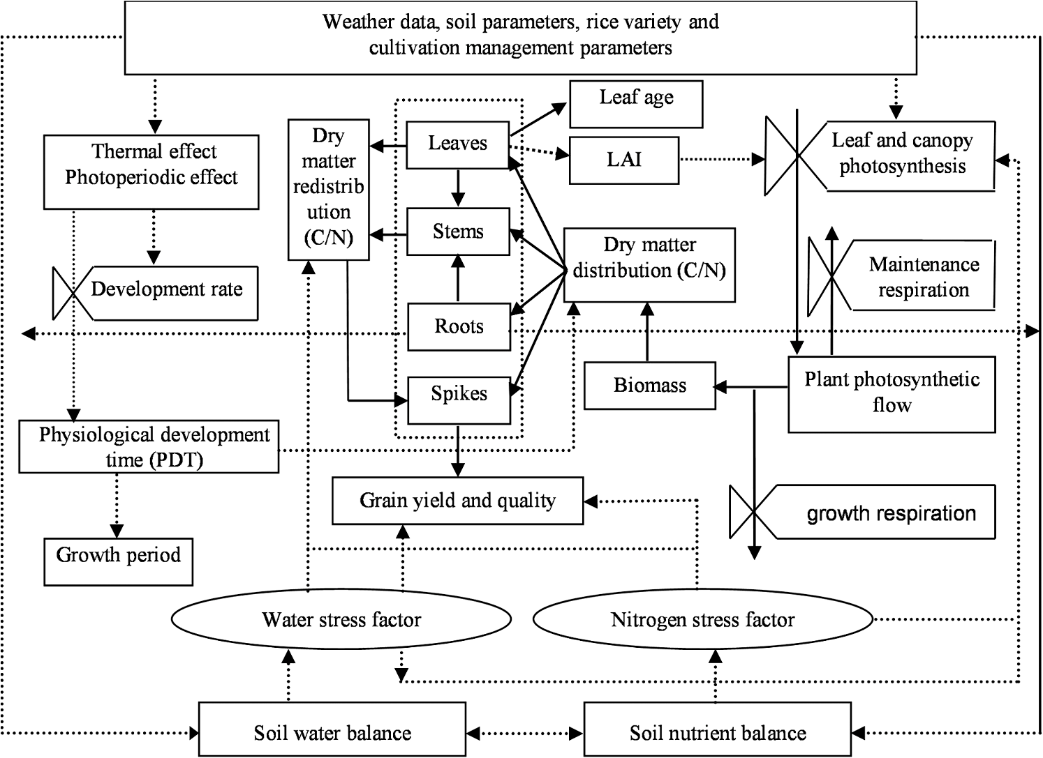
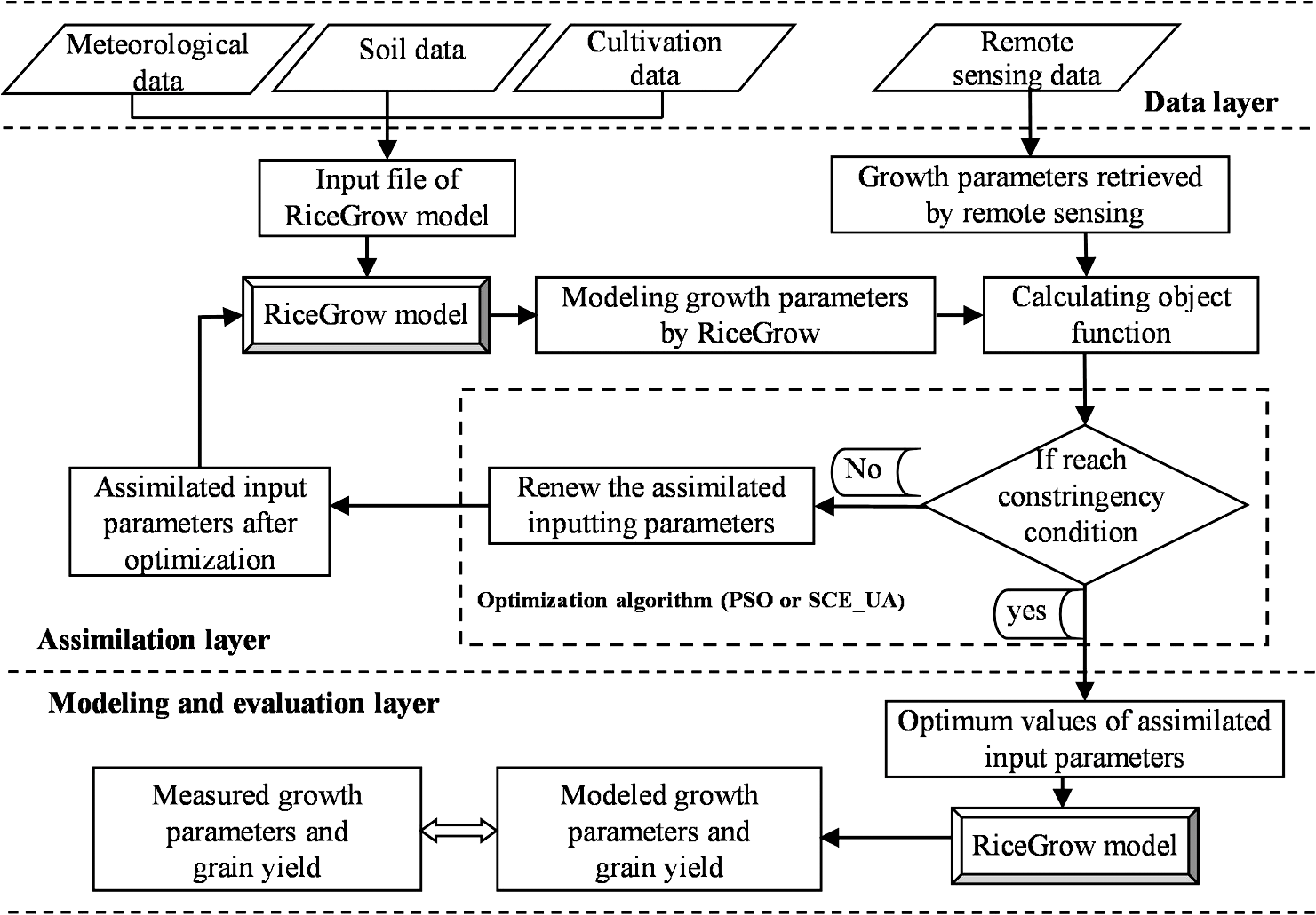
In this study, $m = (2 n + 1)$ , $n$ stands for the number of assimilating parameters, and $p$ was determined as 2.³⁰ The PSO algorithm was compared with the SCE-UA optimization algorithm.

2.5.

Objective Functions

Objective functions are usually used to reflect the differences between the remotely sensed and simulated LAI/LNA values, which determines whether the optimization algorithm (PSO or SCE-UA) had obtained the optimum assimilated input parameters. Here, two different objective functions were developed by using one growth parameter (LAI or LNA) or two growth indexes (LAI and LNA) jointly as the assimilation parameter.

When only LAI or LNA was used as the assimilation parameter, the objective functions were as follows:³¹

Eq. (11)

J = \sum_{i = 1}^{N} | LAI r s, i - LAI m, i | or J = \sum_{i = 1}^{N} | LNA r s, i - LNA m, i | .

When LAI and LNA were used jointly as the assimilation parameter, the $J$ function was used to determine the weighted sum of the square errors of LAI and LNA between RS measurements and RiceGrow simulations. To separate the different effects of LAI and LNA, their weights are considered inversely proportional to the errors of the retrieved LAI and LNA.¹⁴ The $J$ function is calculated as follows:

Eq. (12)

J = \sum_{i = 1}^{N} \frac{{(LAI r s, i - LAI m, i)}^{2}}{Δ_{LAI r s}^{2}} + \sum_{i = 1}^{N} \frac{{(LNA r s, i - LNA m, i)}^{2}}{Δ_{LNA r s}^{2}},

where

J

is the value of the objective function, and

N

is the total number of RS estimation.

LAI r s

and

LNA r s

are the LAI and LNA values retrieved by RS, respectively.

LAI m

and

LNA m

are the corresponding LAI and LNA values simulated by RiceGrow model at the same time RS is conducted.

Δ_{LAI r s}

and

Δ_{LNA r s}

are the standard deviations of LAI and LNA by RS.

2.6.

Rice Growth Model (RiceGrow)

2.6.1.

Brief description of RiceGrow

The RiceGrow model, a process based on the rice growth model, was developed from systematic and comprehensive studies on aspects of the rice cultivation system, such as the mechanisms and relationships among rice growth, climate, soil, and management technology (Fig. 1). The model is composed of seven submodels, including phenology, photosynthesis biomass production, biomass partitioning, yield, quality, and water/nitrogen relationships. Eight genotype-specific parameters relating to rice yield were used: temperature sensitivity, photoperiod sensitivity, optimum temperature, intrinsic earliness (for phonological development), basic filling factor, maximum ${CO}_{2}$ assimilation rate, potential partitioning index for panicle, and potential relative growth rate for LAI. The submodel equations of the RiceGrow model have been exhaustively described in a previous publication by Tang et al.³² The genetic and cultivar ecotype parameters of RiceGrow were adjusted by the trial and error method³³ according to characteristics of the rice cultivars and experimental treatments from the previous experiments,³² which ensure the good predictability and applicability of RiceGrow at various ecosites. The RiceGrow model also could reliably simulate the dynamic processes of rice growth, development, and yield with data from experiments 1, 2, and 3 by validation analysis. The key model state variables LAI and LNA were selected as the coupling parameters for RiceGrow and RS, which not only could express rice growth conditions, but were also directly related to the final grain yield. In addition, data for both of these parameters could be retrieved by RS successfully.³⁴^,³⁵ Sowing date, seeding rate, and nitrogen rate, which are generally difficult to obtain accurately at the regional scale, were chosen as the assimilating parameters of the RiceGrow model.

Fig. 1

Modular structure of the RiceGrow model.

2.6.2.

Crop model input data acquisition

Meteorological data, including daily maximum temperature (°C), daily minimum temperature (°C), sunshine hours (h), and daily rainfall (mm), were acquired from the Weather Bureau of Rugao. The soil data for the study area was obtained from a soil dataset or chemical analysis, including soil thickness (cm), physical clay content (%), bulk density ( ${g cm}^{- 3}$ ), field capacity ( ${cm}^{3} {cm}^{- 3}$ ), wilting humidity ( ${cm}^{3} {cm}^{- 3}$ ), saturated water content ( ${cm}^{3} {cm}^{- 3}$ ), actual water content ( ${cm}^{3} {cm}^{- 3}$ ), saturated hydraulic conductivity ( ${mm d}^{- 1}$ ), organic matter ( ${g kg}^{- 1}$ ), total nitrogen ( ${g kg}^{- 1}$ ), nitrate ( ${mg kg}^{- 1}$ ), ammonium ( ${mg kg}^{- 1}$ ), phosphorus ( ${mg kg}^{- 1}$ ), potassium ( ${mg kg}^{- 1}$ ), and other physical parameters. Geographic information, such as field boundary, was determined using the GPS Pathfinder GPS achiever (Trimble Navigation Ltd., Sunnyvale, California).

3. Results

3.1.

Process of Coupling Remotely Sensed Information and RiceGrow Model

The initialization (assimilation) strategy was adopted to achieve the integration of RS information with the RiceGrow model (Fig. 2). During the assimilation process, the initial input parameters of RiceGrow (sowing/transplanting date, sowing rate, and nitrogen rate) were adjusted constantly until the remotely sensed LAI and LNA values gradually approached those simulated by the RiceGrow model. When the difference between the estimated and simulated values reached the minimum, the input parameters (sowing/transplanting date, sowing rate, and nitrogen rate) were considered to be optimized and then used in the reinitialized RiceGrow model. In this manner, the prediction of rice growth indices and grain yield could be improved based on the RiceGrow model. An optimization algorithm (PSO or SCE-UA) was also used to improve efficiency of the iterative process and determine when the iterative process was terminated in the assimilation process. The integrating process was divided into three layers, including the data layer, assimilation layer, and modeling and evaluation layer.

Fig. 2

Flow chart of coupling remote sensing information and the RiceGrow model.

3.2.

Assimilated Input Parameters and Assimilation Parameter of RS and Crop Model

The selection of input parameters for assimilating should consider whether they have major impacts on the crop model, have large spatial variability in a certain region, and are difficult to obtain accurately.⁴ Accordingly, three rice cultivation management parameters, including sowing/transplanting date, sowing rate, and nitrogen rate, were chosen as the assimilated input parameters. The assimilation parameter is the agronomic parameter serving as the comparative object, which can be estimated and simulated by RS and crop model simultaneously in the assimilation process. In general, those crop growth indices that can be retrieved effectively by RS and are sensitive to the assimilated input parameters are selected as the assimilation parameter.³⁶ In this paper, LAI and LNA together were determined as the assimilation parameter through simple PS analysis.

In the PS analysis, two of three assimilated input parameters were fixed, while the third one was changed in three levels at each time; the LAI and LNA values were simulated accordingly by the RiceGrow model (Fig. 3). The sensitivity of each parameter (LAI or LNA) to the assimilated input parameters was calculated according to Eq. (2). The results showed that the PS of LAI to the three assimilated input parameters, sowing date, sowing rate, and nitrogen rate, were 38.6, 15.9, and 14.0%, and that of LNA were 48.4, 18.1, and 17.4%, respectively. Thus, the three input parameters, sowing date, sowing rate, and nitrogen rate, had major impacts on the RiceGrow model, and LNA was somewhat more sensitive than LAI. Overall, both LAI and LNA were found to be a suitable assimilation parameter alone or jointly.

Fig. 3

Sensitivity analysis of leaf area index (LAI) and leaf nitrogen accumulation (LNA) values simulated by the RiceGrow model to varied values of input parameters of sowing date, sowing rate, nitrogen rate.

3.3.

Validation Runs

3.3.1.

Verification of the assimilation technology

The feasibility of an assimilation technique can be tested by verifying whether it can retrieve the initial input parameters that were used to drive the crop model when the growth parameters simulated by the forward running model are used as the external assimilation data.³⁷ Therefore, data from two treatments (N1D3 and N4D4) in experiment 3, which had clear differences, were used to verify the assimilation procedure in the present paper. First, the RiceGrow model was run forward with the sowing/transplanting date, sowing rate, and nitrogen rate of these treatments, and the simulated daily LAI and LNA were obtained. The developed RS-RiceGrow assimilation model was then run to invert the corresponding initial input parameters with the simulated LAI and LNA serving as external assimilation data. Finally, the differences between the inverted and input parameters were analyzed (Table 2).

Table 2

Differences between the initialized parameters based on the remote sensing (RS)-RiceGrow assimilation model and the original input parameters.

Assimilation parameter	Sowing/transplanting date (day)		Sowing rate (%)		Nitrogen rate (%)
Assimilation parameter	SCE-UA	PSO	SCE-UA	PSO	SCE-UA	PSO
LAI	$- 1$	$- 1$	$- 5.16$	$- 1.8$	$- 5.86$	$- 5.18$
LAI	$- 2$	$- 2$	6.91	6.89	4.7	6.83
LNA	0	$- 1$	$- 9.45$	3.05	$- 9.76$	$- 1.45$
LNA	0	$- 1$	$- 5.63$	1.02	4.26	7.37
LAI and LNA	$- 1$	$- 1$	$- 1.19$	1.94	$- 6.87$	$- 1.8$
LAI and LNA	0	$- 1$	4.87	0.84	7.07	5.67

Note: SCE-UA, shuffled complex evolution-University of Arizona algorithm; PSO, particle swarm optimization algorithm.

The results showed that the RMSE values of three initial parameters between the retrieved and actual values were 1.00 d, $5.42 kg {hm}^{- 2}$ , and $26.57 kg {hm}^{- 2}$ based on the SCE-UA algorithm, while they were 1.22 d, $2.59 kg {hm}^{- 2}$ , and $16.44 kg {hm}^{- 2}$ based on the PSO algorithm, respectively, after running the model 10 times. Moreover, different assimilation parameters also affected the assimilation accuracy. The RMSE values for three initial parameters were 1.58 d, $4.37 kg {hm}^{- 2}$ , and $20.86 kg {hm}^{- 2}$ ; 0.71 d, $5.56 kg {hm}^{- 2}$ , and $25.00 kg {hm}^{- 2}$ ; and 0.87 d, $2.05 kg {hm}^{- 2}$ , and $20.13 kg {hm}^{- 2}$ when using LAI, LNA, and LAI and LNA jointly as the assimilation parameter, respectively. This result indicated that there were no significant differences in sowing date inverting based on the SCE-UA or PSO algorithm; however, the PSO algorithm was more suitable for sowing rate and nitrogen rate retrieval. In addition, the combination of LAI and LNA performed better than each alone as the assimilation parameter in terms of accuracy. In general, the developed assimilation technique was determined to be reliable.

3.3.2.

Field scale validation runs

The retrieved LAI/LNA from experiments 1 and 2 based on field spectral measurements were used to analyze initialization with the input parameters (sowing date/transplanting date, sowing rate, and nitrogen rate) of the RiceGrow model, and different optimization algorithms (PSO and SCE-UA) and assimilation parameters were further compared (Table 3). The results showed that the best assimilation results were obtained when LAI and LNA jointly served as the assimilation parameter based on the PSO optimization algorithm, with RMSE values for sowing date/transplanting date, sowing rate, and nitrogen rate of 3.33 d, $8.57 kg {hm}^{- 2}$ , and $7.99 kg {hm}^{- 2}$ for experiment 1 and 5.75 d, $10.09 kg {hm}^{- 2}$ , and $9.56 kg {hm}^{- 2}$ for experiment 2, respectively. These results were consistent with the results of the initial validation runs above. In addition, the PSO algorithm had a better running efficiency with the faster average calculation time of 39.94 s than that of the SCE-UA algorithm at 87.45 s.

Table 3

Inversion of initialization model parameters by coupling RS and the RiceGrow based on ground RS data.

				Relative error			Root mean square error
	Optimization algorithm	Combination point	Sowing/transplanting Date (day)	Sowing rate (%)	Nitrogen rate (%)	Sowing/transplanting Date (day)	Sowing rate ( $kg \cdot {hm}^{- 2}$ )	Nitrogen rate ( ${kg hm}^{- 2}$ )
Experiment 1	SCE-UA	LAI	$- 4.33$	13.73	$- 13.58$	4.47	9.89	49.16
		LNA	$- 6.5$	16.79	$- 11.88$	5.48	12.46	39.01
		$LAI + LNA$	4	$- 10.67$	$- 8.49$	3.46	9.55	34.48
	PSO	LAI	$- 3.33$	$- 9.03$	$- 8.07$	3.83	11.38	10.83
		LNA	$- 3$	11.63	9.03	4.75	14.2	10.46
		$LAI + LNA$	2.66	8.48	7.58	3.33	8.57	7.99
Experiment 2	SCE-UA	LAI	$- 5.34$	13.84	$- 18.72$	5.02	11.71	61.02
		LNA	$- 5.83$	$- 16.29$	$- 14.68$	6.47	11.48	43.87
		$LAI + LNA$	4.16	$- 12.76$	$- 11.44$	5.49	10.34	47.4
	PSO	LAI	$- 3.83$	8.62	$- 9.77$	4.66	11.23	14.25
		LNA	$- 5.67$	8.85	8.51	4.08	12.57	11.09
		$LAI + LNA$	3.16	7.91	$- 7.67$	5.75	10.09	9.56

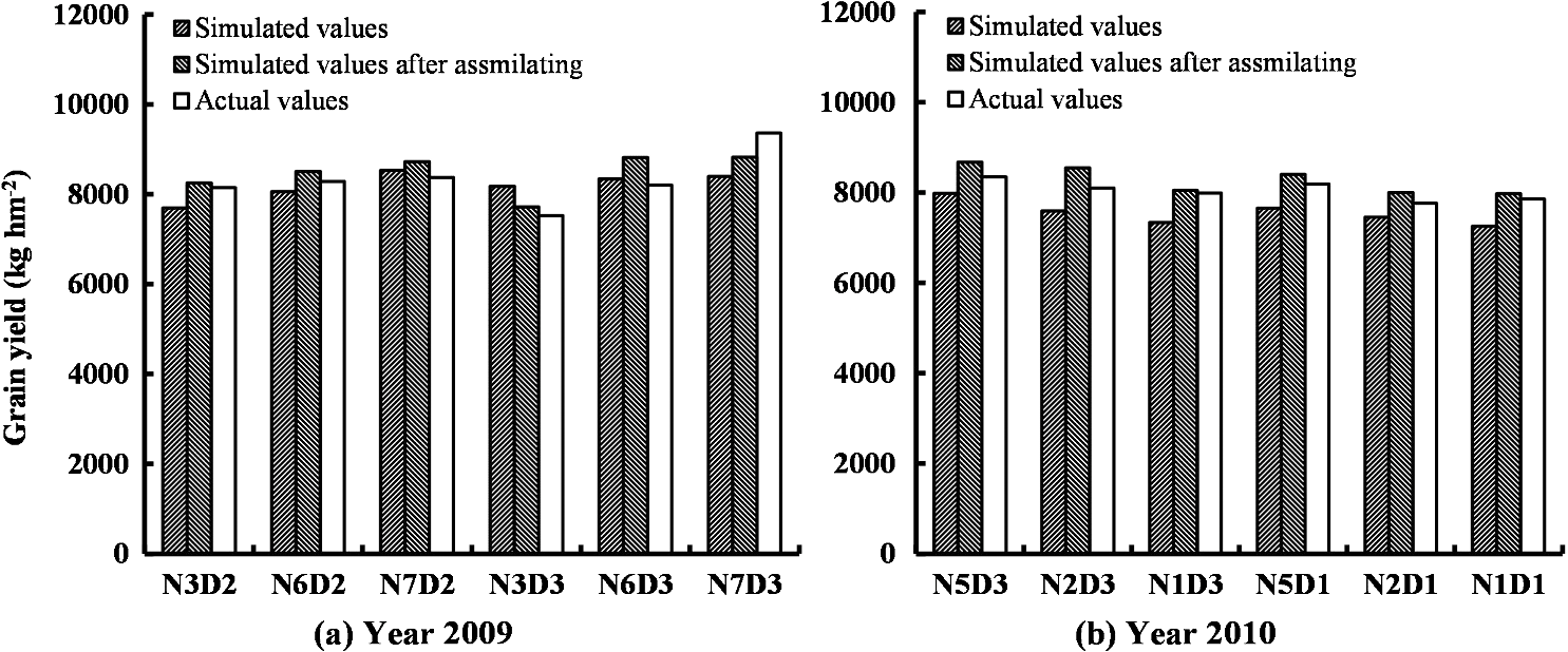
Therefore, LAI and LNA dynamics and grain yield of rice were simulated by the RS-RiceGrow assimilation model based on the PSO algorithm and the optimal assimilation parameter (LAI and LNA). The results showed that the RMSE and RE values between the simulated and measured values of LAI, LNA, and grain yield were 1.01, $0.59 g m^{- 2}$ , $335.70 kg {hm}^{- 2}$ , and 0.19, 0.11, and 2.47%, respectively (Figs. 4 and 5). Meanwhile, the corresponding values of RMSE and RE were 1.25, $1.24 {g m}^{- 2}$ , $516.83 kg {hm}^{- 2}$ , and 0.28, 0.18, and $- 3.61 %$ , respectively, based on the RiceGrow model alone. Thus, the assimilation model based on coupling RS and RiceGrow model improved prediction accuracy and could be utilized in a practical application.

Fig. 4

Comparisons of simulated and measured LAI and LNA values by RiceGrow before and after assimilation based on data from experiment 2.

Fig. 5

Comparisons of simulated and measured grain yield by RiceGrow before and after assimilation based on data from experiments 1 and 2.

3.3.3.

Regional-scale validation runs

The RS-RiceGrow assimilation model based on the PSO algorithm was further tested on the whole study area. The sowing/transplanting period, nitrogen rate and seeding rate, and grain yield of rice in the study area were inverted and simulated as shown in Fig. 6. The results showed that in the eastern area of Rugao City, the date of transplanting was relatively early with a higher level of nitrogen application and seeding rates and grain yield. Additionally, the planting method in Changjiang Town located in the southern area of Rugao (farm) was direct seeding, while other towns mainly used transplanting. The sowing date for Changjiang Town and transplantion date for other towns are shown in Fig. 6. These results were consistent with the actual field surveys. Compared to the ground measured values, the assimilation model had a relatively high simulation precision, with the inversion RMSE and RE values of sowing/transplanting date, sowing and nitrogen rates, grain yield calculated as 5.76 d, $13.41 kg {hm}^{- 2}$ , $58.34 kg {hm}^{- 2}$ , and $426.11 kg {hm}^{- 2}$ ; 6.16 d, 12.76%, 11.43%, and 7.45%, respectively. The predicted average yield and total production of rice in Rugao City were $8220.93 kg {hm}^{- 2}$ and 47.81 million kilograms, which were close to the officially reported values of $8460 kg {hm}^{- 2}$ and 42 to 45 million kilograms in 2009. The slightly higher predicted total production compared to actual values may be attributed to error from the process of extracting the rice planting area.

Fig. 6

Spatial distributions of initialized input parameters and simulated grain yields in the study area.

4. Discussion

Integrating RS and a crop growth model is a robust way to estimate regional crop yield, and SCE-UA has been a widely used optimization algorithm for this purpose. However, many more parameters must be determined, which would increase the complexity of calculations, and repeated testing is needed before SCE-UA can be used effectively.¹⁸ By comparison, the less complex PSO algorithm can be run with a simple encoded mode and without genetic operators, such as selection, crossover, and mutation.³⁸ Therefore, a new PSO optimization algorithm was introduced and compared with SCE-UA in the present paper. The results showed that there were no significant differences in inverting sowing data between the SCE-UA and PSO algorithms. However, the PSO algorithm had a higher retrieval precision for sowing rate and nitrogen rate than did SCE-UA. Moreover, the PSO algorithm also had better precision for assimilating initial input parameters and grain yield simulation when used at the regional scale. Furthermore, there was a higher running speed with the same number of cycles for the PSO algorithm, indicating that it is more suitable for use on a regional scale than SCE-UA.

Regardless of the optimization algorithm used, the assimilation accuracy of initial input parameters of crop model is significantly influenced by the error of external assimilation parameters. The assimilation results from ground-based and spaceborne RS data in this study confirmed this idea and were consistent with previous observations.³⁹ Thus, the accuracy of agronomic parameter estimation based on RS should be further improved to facilitate the effective integration of RS and crop growth models, which may be achieved by adopting RS images with high spatial and spectral resolutions and utilizing radiative transfer models to enhance the mechanistic theory of parameter inversion. Meanwhile, the performance of an assimilation algorithm and its parameters setting also has some impact on the assimilation accuracy, and the method for setting those parameters should be further examined in future studies. Moreover, the assimilating strategy used in this paper is based on the assumption that RS observations can better reflect the objective reality than the crop growth model. Thus, combining the assimilation strategy and the updating strategy in further work would be a promising approach to improve the prediction accuracy of agronomic parameters, since the updating strategy would simultaneously remove the errors from both RS observation and crop growth simulation.⁴⁰ A more routine use of combined RS and crop modeling techniques would improve our ability to estimate regional rice grain yield predictions. It should be noted that the RS-RiceGrow assimilation model developed in the study is also based on the accuracy and reliability of the RiceGrow model. Therefore, finding certain nondeterminant factors of the RiceGrow model and improving accuracy by integrating RS would be key points in further study.

Numerous previous studies have used LAI as the assimilation parameter,¹⁴^,³⁹ but additional physiological parameters have been successfully estimated with the development of RS technology.²⁴ Therefore, LAI and LNA alone or jointly were compared as the assimilation parameter of RS and the crop model in this study. The results showed that the rank order of different assimilation parameters based on assimilation precision was LAI and LNA jointly $> LNA > LAI$ , indicating that using multiple physiological parameters as the assimilation parameter can improve the acquisition of initial model input parameters. This is because LAI and LNA jointly can well reflect both crop canopy population status and nitrogen nutrition status. Fortunately, estimating multiple physiological parameters from one remote sensor (or one image) can be achieved with the development of multipectral or hyperspectral RS technology.²⁴^,²⁵

The integrated model developed in this paper can be run feasibly within a small study area by a single commodity computing system. However, processing increasingly complex RS and data assimilation strategies will become unfeasible for an average computer. This implies that state-of-the-art-models will typically be slightly beyond the computing capability of the current commodity system, thereby warranting the need for parallel or distributed processing, which would allow multiple computer nodes to cooperate on a common problem.³⁶ The use of multiple simultaneous computing nodes offers the potential for enhanced agro-ecosystem modeling. However, the scope of this potential remains to be determined in further research.

5. Conclusion

A regional rice grain yield prediction technique was proposed by integration of ground-based and spaceborne RS data with the RiceGrow model through a new PSO algorithm with LAI and LNA jointly as the assimilation parameter in the present paper. LAI together with LNA as the integrated parameter performed better than each alone for crop model parameter initialization. PSO also performed better than SCE-UA in terms of running efficiency and assimilation results, indicating that PSO is a reliable optimization method for assimilating RS information and the crop growth model. The integrated model showed good accuracy of prediction for rice growth parameters and grain yield in both the field and regional scales and was demonstrated to be an improved approach for regional crop yield assessment.

Acknowledgments

This research was supported by National Natural Science Foundation of China (31371535), National 863 High-tech Program (2013AA102301 and 2011AA100703), the Special Fund for Agro-scientific Research in the Public Interest (201303109), the Science and Technology Support Program of Jiangsu (BE2010395, BE2011351, and BE2012302), and the Priority Academic Program Development of Jiangsu Higher Education Institutions, China.

References

1.

FAO, “Food and agricultural commodities production,” (2011) http://faostat.fao.org/site/339/default.aspx September ). 2011). Google Scholar

2.

R. Singhet al., “Small area estimation of crop yield using remote sensing satellite data,” Int. J. Remote Sens., 23 (1), 49 –56 (2002). http://dx.doi.org/10.1080/01431160010014756 IJSEDK 0143-1161 Google Scholar

3.

W. G. M. BastiaanssenS. Ali, “A new crop yield forecasting model based on satellite measurements applied across the Indus Basin, Pakistan,” Agric. Ecosyst. Environ., 94 (3), 321 –340 (2003). http://dx.doi.org/10.1016/S0167-8809(02)00034-8 AEENDO 0167-8809 Google Scholar

4.

S. MoulinA. BondeauR. Delecolle, “Combining agricultural crop models and satellite observations: from field to regional scales,” Int. J. Remote Sens., 19 (6), 1021 –1036 (1998). http://dx.doi.org/10.1080/014311698215586 IJSEDK 0143-1161 Google Scholar

5.

T. Hodgeset al., “Using the CERES-Maize model to estimate production for the U.S. Cornbelt,” Agric. For. Meteorol., 40 (4), 293 –303 (1987). http://dx.doi.org/10.1016/0168-1923(87)90043-8 0168-1923 Google Scholar

6.

M. Cabelguenneet al., “Calibration and validation of EPIC for crop rotations in southern France,” Agric. Syst., 33 (2), 153 –171 (1990). http://dx.doi.org/10.1016/0308-521X(90)90078-5 AGSYD5 0308-521X Google Scholar

7.

R. A. BrownN. J. Rosenberg, “Sensitivity of crop yield and water use to change in a range of climatic factors and

{CO}_{2}

concentrations: a simulation study applying EPIC to the central USA,” Agric. For. Meteorol., 83 (3–4), 171 –203 (1997). http://dx.doi.org/10.1016/S0168-1923(96)02352-0 0168-1923 Google Scholar

8.

S. Assenget al., “Performance of the APSIM-wheat model in Western Australia,” Field Crop Res., 57 (2), 163 –179 (1998). http://dx.doi.org/10.1016/S0378-4290(97)00117-2 FCREDZ 0378-4290 Google Scholar

9.

B. Simaneet al., “Application of a crop growth model (SUCROS-87) to assess the effect of moisture stress on yield potential of durum wheat in Ethiopia,” Agric. Syst., 44 337 –353 (1994). http://dx.doi.org/10.1016/0308-521X(94)90226-6 AGSYD5 0308-521X Google Scholar

10.

R. Faivreet al., “Spatialising crop models,” Agronomie, 24 205 –217 (2004). http://dx.doi.org/10.1051/agro:2004016 AGRNDZ 0249-5627 Google Scholar

11.

R. Delecolleet al., “Remote sensing and crop production models: present trends,” ISPRS J. Photogramm., 47 (2–3), 145 –161 (1992). http://dx.doi.org/10.1016/0924-2716(92)90030-D IRSEE9 0924-2716 Google Scholar

12.

P. C. Doraiswamyet al., “Crop condition and yield simulations using Landsat and MODIS,” Remote Sens. Environ., 92 (4), 548 –559 (2004). http://dx.doi.org/10.1016/j.rse.2004.05.017 RSEEA7 0034-4257 Google Scholar

13.

O. Abou-IsmailJ. F. HuangR. C. Wang, “Rice yield estimation by integrating remote sensing with rice growth simulation model,” Pedosphere, 14 519 –526 (2004). PDOSEA Google Scholar

14.

L. Denteet al., “Assimilation of leaf area index derived from ASAR and MERIS data into CERES-Wheat model to map wheat yield,” Remote Sens. Environ., 112 (4), 1395 –1407 (2008). http://dx.doi.org/10.1016/j.rse.2007.05.023 RSEEA7 0034-4257 Google Scholar

15.

J. Q. Renet al., “Integrating remotely sensed LAI with EPIC model based on global optimization algorithm for regional crop yield assessment,” in Proc. of IEEE Int. Geoscience and Remote Sensing Symp. (IGARSS), 2147 –2150 (2010). Google Scholar

16.

H. L. FangS. L. LiangG. Hoogenboom, “Integration of MODIS LAI and vegetation index products with the CSM-CERES-Maize model for corn yield estimation,” Int. J. Remote. Sens., 32 (4), 1039 –1065 (2011). http://dx.doi.org/10.1080/01431160903505310 IJSEDK 0143-1161 Google Scholar

17.

Y. Huanget al., “Predicting winter wheat growth based on integrating remote sensing and crop growth modeling techniques,” Acta Ecologica Sinica, 31 1073 –1084 (2011). Google Scholar

18.

Q. Y. DuanS. SorooshianV. K. Gupta, “Optimal use of the SCE_UA global optimization method for calibrating watershed models,” J. Hydrol., 158 (3–4), 265 –284 (1994). http://dx.doi.org/10.1016/0022-1694(94)90057-4 JHYDA7 0022-1694 Google Scholar

19.

G. X. Bai, “China environmental and disaster monitoring and forecasting small satellite—HJ-1A/B,” Aerosp. China, 5 10 –15 (2009). Google Scholar

20.

(2006). Google Scholar

21.

Y. Shenet al., “Rational consideration about construction land expansion of Changsha urban area in the last ten years,” Geogr Geo-Info. Sci., 23 27 –30 (2007). 1365-8816 Google Scholar

22.

C. HuangL. S. DavisJ. R. G. Townshend, “An assessment of support vector machines for land cover classification,” Int. J. Remote. Sens., 23 (4), 725 –749 (2002). http://dx.doi.org/10.1080/01431160110040323 IJSEDK 0143-1161 Google Scholar

23.

G. M. FoodyA. Mathur, “A relative evaluation of multiclass image classification by support vector machines,” IEEE Trans. Geosci. Remote Sens., 42 (6), 1335 –1343 (2004). http://dx.doi.org/10.1109/TGRS.2004.827257 IGRSD2 0196-2892 Google Scholar

24.

L. H. Xueet al., “Monitoring leaf nitrogen status in rice with canopy spectral reflectance,” Agron. J., 96 (1), 135 –142 (2004). http://dx.doi.org/10.2134/agronj2004.0135 AGJOAT 0002-1962 Google Scholar

25.

Y. C. Tianet al., “Quantitative relationships between hyper-spectral vegetation indices and leaf area index of rice,” Chinese J. Appl. Ecol., 20 (7), 1685 –1690 (2009). Google Scholar

26.

I. Numataet al., “Evaluation of hyperspectral data for pasture estimate in the Brazilian Amazon using field and imaging spectrometers,” Remote Sens. Environ., 112 (4), 1569 –1583 (2008). http://dx.doi.org/10.1016/j.rse.2007.08.014 RSEEA7 0034-4257 Google Scholar

27.

P. D. JamiesonJ. R. PorterD. R. Wilson, “A test of the computer simulation model ARCWHEAT1 on wheat crops grown in New Zealand,” Field Crops Res., 27 (4), 337 –350 (1991). http://dx.doi.org/10.1016/0378-4290(91)90040-3 FCREDZ 0378-4290 Google Scholar

28.

J. KennedyR. Eberhart, “Particle swarm optimization,” in IEEE Int. Conf. on Neural Networks Proc. (ICNN 95), 1942 –1948 (1995). Google Scholar

29.

R. C. EberhartY. H. Shi, “Particle swarm optimization: developments, applications and resources,” in IEEE Proc. Congress on Evolutionary Computation, 81 –86 (2001). Google Scholar

30.

Q. Y. DuanV. K. GuptaS. Sorooshian, “Shuffled complex evolution approach for effective and efficient global minimization,” J. Optim. Theory Appl., 76 (3), 501 –521 (1993). http://dx.doi.org/10.1007/BF00939380 JOTABN 0022-3239 Google Scholar

31.

Y. X. Zhao, “Study on the method of combination of remote sensing and crop model and its application,” Peking University, (2005). Google Scholar

32.

L. Tanget al., “RiceGrow: a rice growth and productivity model,” NJAS-Wagen. J. Life Sci., 57 (1), 83 –92 (2009). http://dx.doi.org/10.1016/j.njas.2009.12.003 1573-5214 Google Scholar

33.

J. PanY. ZhuW. Cao, “Modeling plant carbon flow and grain starch accumulation in wheat,” Field Crop Res., 101 (3), 276 –284 (2007). http://dx.doi.org/10.1016/j.fcr.2006.12.005 FCREDZ 0378-4290 Google Scholar

34.

R. Darvishzadehet al., “LAI and chlorophyll estimation for a heterogeneous grassland using hyperspectral measurements,” ISPRS J. Photogramm., 63 (4), 409 –426 (2008). http://dx.doi.org/10.1016/j.isprsjprs.2008.01.001 IRSEE9 0924-2716 Google Scholar

35.

W. Fenget al., “Monitoring leaf nitrogen status with hyperspectral reflectance in wheat,” Eur. J. Agron., 28 (3), 394 –404 (2008). http://dx.doi.org/10.1016/j.eja.2007.11.005 EJAGET 1161-0301 Google Scholar

36.

W. A. Dorigoet al., “A review on reflective remote sensing and data assimilation techniques for enhanced agroecosystem modeling,” Int. J. Appl. Earth Obs., 9 (2), 165 –193 (2007). http://dx.doi.org/10.1016/j.jag.2006.05.003 0303-2434 Google Scholar

37.

M. GuerifC. L. Duke, “Adjustment procedures of a crop model to the site specific characteristics of soil and crop using remote sensing data assimilation,” Agric. Ecosyst. Environ., 81 57 –69 (2000). http://dx.doi.org/10.1016/S0167-8809(00)00168-7 AEENDO 0167-8809 Google Scholar

38.

Y. Jianget al., “Improved particle swarm optimization for parameter calibration of Xin’anjiang model,” J. Hydraul. Eng., 38 1200 –1206 (2007). JHEND8 0733-9429 Google Scholar

39.

Y. Yanet al., “Methodology of winter wheat yield prediction based on assimilation of remote sensing data with crop growth model,” J. Remote Sens., 10 804 –811 (2006). Google Scholar

40.

A. J. W. de WitC. A. van Diepen, “Crop model data assimilation with the Ensemble Kalman filter for improving regional crop yield forecasts,” Agric. For. Meteorol., 146 (1–2), 38 –56 (2007). http://dx.doi.org/10.1016/j.agrformet.2007.05.004 0168-1923 Google Scholar

Biographies of the authors are not available.

CC BY: © The Authors. Published by SPIE under a Creative Commons Attribution 4.0 Unported License. Distribution or reproduction of this work in whole or in part requires full attribution of the original publication, including its DOI.

Citation Download Citation

Hang Wang, Yan Zhu, Wenlong Li, Weixing Cao, and Yongchao Tian "Integrating remotely sensed leaf area index and leaf nitrogen accumulation with RiceGrow model based on particle swarm optimization algorithm for rice grain yield assessment," Journal of Applied Remote Sensing 8(1), 083674 (18 February 2014). https://doi.org/10.1117/1.JRS.8.083674

Published: 18 February 2014

Access the abstract

JOURNAL ARTICLE
17 PAGES

DOWNLOAD PAPER SAVE TO MY LIBRARY

GET CITATION

CITATIONS

Cited by 44 scholarly publications.

Explore citations on Lens.org

KEYWORDS

Data modeling

Remote sensing

Nitrogen

Particle swarm optimization

Optimization (mathematics)

Particles

Yield improvement

1.

Introduction

2.

Materials and Methods