1.

Introduction

Despite its small area, Slovenia is exceptionally diverse in terms of its physical geography.¹ This is confirmed by the fact that its territory is categorized into various landscape types and regions at the European level.^2–4 The area of Slovenia is on the border of northern and southern climatic division (Fig. 1),⁵ what is another proof of high natural diversity. In classifying Slovenia’s small area with very diverse landscape (that is evident also in a small scale), the question arises whether it is also necessary to take into account natural elements that are commonly known as appropriate for landscape classification at continental or worldwide level (e.g., latitude, climate). One such element is the delayed appearance of phenological phases with regard to vertical and, especially, horizontal distance from the sea (e.g., onset of leafing out and onset of leaf loss). These phenomena are also known as the green wave and brown wave.⁶ Climate (e.g., temperature) is decisive for the development of plants and affects phenology,^7,8 and climate is also an important factor in classification at the smallest scale.⁹ Regarding the significance of other natural elements for spatial classification, climate and the related climatic vegetation zones connected^9,10 are more appropriate for analysis at the continental level, and not for small countries. Judging by climate data—specifically, the ratio between average April and October temperatures, which can show the influence of a continental location or distance from the sea—Slovenia is quite diverse despite its small area ($\mathrm{20,273}{\mathrm{km}}^2$). The ratio between average April and October temperatures in Portorož, where the cool sea prevents rapid warming of the air in early spring, is 0.81, whereas the ratio for Murska Sobota, which lies in the northeast part of the country and where the air warms up more quickly in the spring but also cools off more quickly in the fall, is 1.04.¹¹ Similar differences can be observed between Lisbon, Portugal (0.82) and Kyiv, Ukraine (1.08), for example.¹²

Fig. 1

According to some continental climatic classifications (Ref. 5), Slovenia is situated on the border between northern and southern continental climatic regions.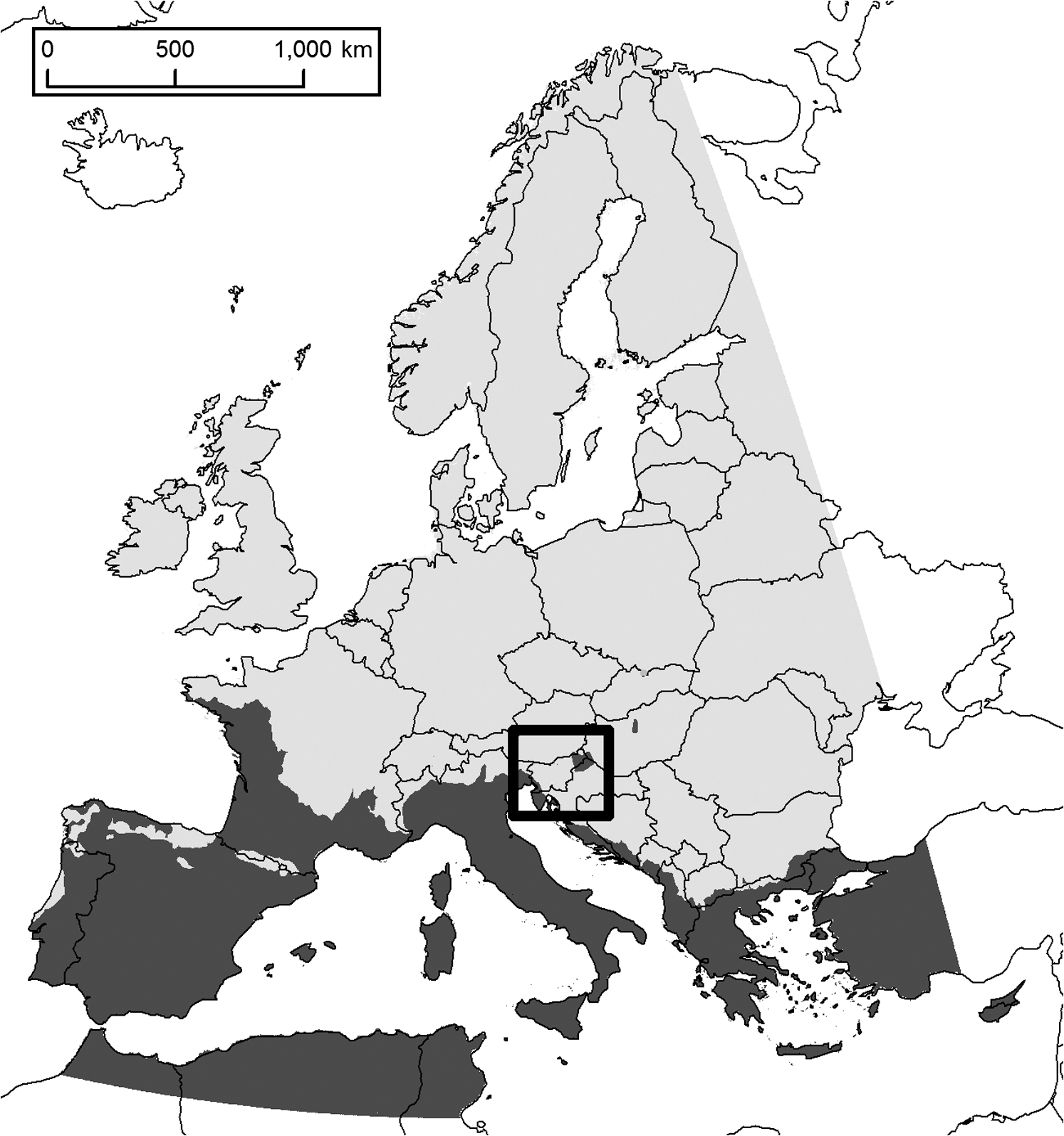

This diversity of Slovenia raises the question whether its territory has an observable delay in phenological events as distance from the sea increases, that is, whether certain natural factors (that are usually variable at greater distance) retain high variation in a small area as well and are also observable in a small area. At the same time, phenological events can be compared with elevation, namely, temperatures change more drastically with elevation than with latitude or distance from the sea. Specifically, change in the vertical direction usually has a greater influence than in the horizontal direction.¹⁰ Because of this it can be expected that changes in phenological phenomena are more distinct in the vertical direction than in the horizontal direction (i.e., with distance from the sea). An important argument for carrying out phenological research with satellite images in Slovenia is that Slovenia is one of the most heavily forested countries in Europe.¹³ Along with this, some farmed areas are being abandoned and becoming forested (again).^14,15

The main goal of this study is to use phenological data (especially on the onset of greenness and greenness decrease) obtained from satellite images to analyze phenological phenomena with regard to distance from the sea and elevation and to examine whether green wave is noticed in vertical and horizontal direction.

1.1.

Remote Sensing and Phenology

The spectral ratio between infrared and red bands has great importance for observing the state of vegetation because vegetation reflects infrared and absorbs red part of the electromagnetic spectrum.¹⁶ The ratio enables observation of changes in structural, phenological, and biophysical parameters between seasons and years.¹⁷ It should also be added that the spectral vegetation indices are more stable across time than individual spectral bands.¹⁸

The main advantage of using remote sensing in phenological studies is the continuous capture of phenological samples in the larger areas and the ability to analyze past periods from archival images.¹⁹ The seasonal sample of variation in areas with vegetation acquired using remote sensing data is defined as landsurface phenology. This kind of phenology differs from the traditional phenology of plants, which deals with life-cycle phenomena (such as flowering, leafing out, and leaf loss) with the help of in situ observation of individual plant species.²⁰ Specifically, remote sensing makes possible the shift from observing individual plants to broader phenological samples of the area.¹⁹ The phenology of entire ecosystems was less studied until the introduction of remote sensing.⁶ Satellite sensors are capable of detecting and measuring changes in the landscape at a broader scale (Fig. 2), which may not coincide with the phenological incidence of individual plants because they describe the state of the entire ecosystem.⁶ Due to this fact landsurface phenology is indicating a mixture of different land covers and is distinct from traditional species-centric phenology.²¹ Such analysis can also be carried out in areas with deficient phenological data.²² Different approaches were used to define the key dates (events) of phenological phenomena in terrain phenology.^6,18,20,23

Fig. 2

Depiction of the onset of greenness increase for West Africa (Ref. 24).

In addition to the method of defining the key dates, there are also several different phenological measures. Phenological measures are divided into three groups: temporal measures, vegetation index measures, and derived measures (Table 1). These measures usually do not directly correspond to an actual phenological phenomenon, but they are indicators of ecosystem dynamics. These phenomena can be detected with satellite observations as a sudden increase in the vegetation index and they signal a change in the ecosystem.⁶

Table 1

Measures derived from vegetation index data (Ref. 6).

Group of metrics	Metric	Phenological interpretation
Temporal vegetation index metrics	Time of onset of greenness	Beginning of measureable photosynthesis
	Time of end of greenness	Cessation of measureable photosynthesis
	Duration of greenness	Duration of photosynthetic activity
	Time of maximum vegetation index	Time of maximum measureable photosynthesis
Vegetation index value metrics	Value of onset of greenness	Level of photosynthetic activity at the beginning of growing season
	Value of end of greenness	Level of photosynthetic activity at the end of growing season
	Value of maximum vegetation index	Maximum measureable level of photosynthetic activity
	Range of vegetation index	Range of measureable photosynthetic activity
Derived metrics	Time-integrated vegetation index	Net primary production
	Rate of greenup	Acceleration of photosynthesis
	Rate of senescence	Deceleration of photosynthesis
	Modality	Periodicity of photosynthetic activity

This article uses measures that could be categorized into the group of temporal measures: we studied the onset of greenness increase, onset of greenness decrease, and duration of the greenness (i.e., vegetation period).

Phenology studies using satellite data go back relatively far. Rouse et al. carried out one of the first studies to determine phenological events using Landsat multispectral scanner (MSS) images.²⁵ This was one of the first studies that used the vegetation index obtained from the red and near-infrared spectrum to define the green wave and brown wave.^6,25 Later, these types of phenomena were comprehensively studied by using data from the advanced very high resolution radiometer (AVHRR)^6,22,26 and the moderate resolution imaging spectroradiometer (MODIS) sensors.^18,27

2.

Data for Analysis

The information useful for regional phenology studies is captured by several satellite systems (Table 2), among which those with higher spatial resolution are especially appropriate for use.¹⁹ Some sensors have more spectral bands than others (e.g., MODIS has more spectral bands in comparison to AVHRR).²⁸

Table 2

Satellite sensors and datasets useful for studying phenological terrain features (Refs. 19 and 29).

For our analysis, we used MODIS satellite products on phenological phenomena (onset of greenness increase and onset of greenness decrease). We also included forest area, and digital elevation model and horizontal distance from the sea (Table 3). All of the layers were masked to exclude nonforest areas. For validation we used phenological data recorded by observers from the network of the Slovenian Environment Agency (code ARSO).³⁰

Table 3

List of data for carrying out the analysis.

2.2.

MODIS Satellite Data and Products

Because of its excellent temporal and good spatial resolution, we used data and products from the MODIS system.³⁷ MODIS is an instrument with high radiometric (12 bit) and spectral resolution: 36 spectral bands in a wavelength range from 0.4 to 14.4 μm. Its spatial resolution is somewhat smaller, at 250 to 1000 m. The MODIS instrument is onboard of two satellites: Terra, which was placed in orbit in December 1999, and Aqua, which was launched in May 2002. Both of them have near-polar orbits, are sun-synchronous, and together they image the entire Earth every one to two days.³⁸

The applicability of products from MODIS satellite images in phenology was extensively studied for North and South America, especially in comparison with aerial photos and terrestrial measurements. It was determined that the vegetation indices calculated from the MODIS images are sensitive to seasonable vegetation variability, land cover, and biophysical parameters.¹⁷ However, it should be noted that vegetation indexes can be different, depending on sensor.³⁹

The product range of the land cover dynamics yearly L3 global 500 m SIN grid, also known as the MODIS global vegetation phenology product, coded MCD12Q2 version 005, shows the course of phenological development of vegetation through the year at the global level. It contains data on the range and value of the enhanced vegetation index and it offers information on vegetation growth, maturity, and aging. Data on the enhanced vegetation index (EVI), calculated from the MODIS product nadir bidirectional reflectance distribution function adjusted reflectance (NBAR), were used to produce the MCD12Q2 data set. NBAR values were calculated from eight daily periods with a spatial resolution of 500 m.³¹ It was proved that product MCD12Q2 can be generally reliable when analyzing crop phenology.⁴⁰

To define the dates of phenological transitions (or phenomena), the level of change in the curve of the model was used.⁴¹ The dates correspond to the time when the degree of change in the EVI value was lowest or greatest. Four transitional phenological events are defined: onset of greenness increase, onset of greenness maximum, onset of greenness decrease, and onset of greenness minimum (Fig. 3).⁴¹ The data layers containing the daily phenological phenomena define the approximate onset and end of the growth period, the length of the growth period, and the time of the greatest value of greenness in the year.

Fig. 3

Phenological events with regard to idealized nadir bidirectional reflectance distribution function adjusted reflectance enhanced vegetation index values: (a) Onset of greenness increase, (b) onset of greenness maximum, (c) onset of greenness decrease, and (d) onset of greenness minimum (Ref. 41).

3.

Analysis

We analyzed the dependence of phenological phenomena on elevation and distance from the sea for the following phenological data for the year 2006: onset of greenness increase [Fig. 4(a)], onset of greenness decrease [Fig. 4(b)], and length of the vegetation period [i.e., difference between onset of greenness decrease and onset of greenness increase; Fig. 4(c)].

Fig. 4

Depiction of onset of greenness increase (a), onset of greenness decrease (b), and length of vegetation period (c) for Slovenia in 2006.

We prepared the data and calculated the correlations using the Idrisi Taiga (version 16.05) and SPSS (version 16.0).

First, we calculated the average value for every phenological data layer and looked for the lowest and highest values. In this way, we obtained a basic overview of the phenomenon (Table 4).

Table 4

Basic statistical features of phenological data from MODIS satellite images (MCD12Q2 data set). Onset of greenness decrease is more variable than onset of greenness increase.

With regard to the average value of all pixels in the data layer, it can be seen that the average onset of greenness increase is the 97th day of the year, or sometime in the beginning of April. Onset of greenness decrease is defined on average on the 218th day of the year, or sometime in August, but its variability is greater than in the previous case. Length of the growing period is defined as the length of the period between leafing out and yellowing of foliage.⁴² In our case, we subtracted the day of the onset of greenness decrease from the day of the onset of greenness increase in order to calculate the length of the vegetative period, a consequence of which is a significantly shorter vegetative period than the actual one. The average length is, thus, 121 days, which is approximately four months.

We analyzed correlations with elevation and distance from the sea for each phenological data layer (onset of greenness increase, onset of greenness decrease, and length of the vegetation period). The correlation indicator was selected after we checked whether the variables had a normal distribution (by calculating the coefficients of skewness and kurtosis). Variables that have a normal distribution normally have coefficients of skewness and kurtosis between $-1$ and 1. The basic features of certain variables in the MODIS data layers show (Table 5) that not all of them have a normal distribution, which prevents the use of parametric methods (e.g., calculating the Pearson correlation coefficient and the coefficient of partial correlation) for all variables. Therefore, we calculated Spearman’s correlation coefficient (Table 6) because this does not require a normal distribution and allows a comparison of correlation among all variables. Because the number of units (pixels) was too large, we randomly divided pixels in 10 sets. In each one of them there were $\sim 10\%$ of all pixels. We then calculated Spearman coefficient for each of the 10 sets; all the pixels in our study area were, thus, included in the calculation.

Table 5

Basic statistical features of MODIS data (standardized values). The number of pixels is 961,570. There are no missing values. Non-normal data distribution, which is determined from the coefficients of skewness and kurtosis, prevents the use of parametric statistical methods.

Table 6

Maximum and minimum values of Spearman’s correlation coefficients based on 10 samples with 10% of all pixels in each sample being statistically significant at p<0.01. This is a two-tailed test. Onset of greenness increase and elevation correlate most strongly (>0.7. The negative correlation coefficient between onset of greenness increase and distance from the sea is partially a consequence of the fact that in western Slovenia (which is relatively close to the sea), the land is considerably higher than in the east and northeast. Onset of greenness decrease correlates very weakly with elevation and also with distance from the sea. As a result, the correlation of the vegetation period with these data layers is also low.

As can be seen in Table 6, there is a high positive correlation between onset of greenness increase and elevation ($>0.7$) and, to a considerably less extent, also the correlation between elevation and vegetation period ($<0.4$). The latter is lower than the former primarily due to the small correlation between elevation and onset of greenness decrease, which amounts from $-0.15$ up to $-0.16$ and is properly negative because the vegetation period is shorter with increasing elevation. On the basis of these results, relative strong vertical green wave can be confirmed, but not also vertical brown wave.

Because elevation rises sharply across the Karst rim with distance from the sea (toward the northeast), and then gradually decreases from the Dinaric karst plateaus onward (Fig. 5), it is necessary to exclude the influence of elevation for suitably calculating the correlation of phenological phenomena with distance from the sea. Spearman’s correlation coefficient points to the decrease in elevation with distance from the sea; its values are from $-0.25$ to $-0.27$, which is statistically significant. Unfortunately, the non-normal distribution of certain data makes it impossible to calculate a partial correlation, which would provide more reliable results. The fact that the onset of greenness increase occurs earlier with distance from the sea and the onset of greenness decrease occurs later is, therefore, probably a result of higher elevation in western Slovenia. Because of this, the vegetation period becomes longer with distance from the sea in our data.

Fig. 5

: Elevation (a) and distance from sea (b) in Slovenia and surroundings.

In order to exclude the influence of altitude, correlation between phenological phenomena and distance from the sea only for pixels with similar elevation (Table 7) was calculated. It is evident that the correlations for most of the elevation classes are $<-0.3$ and only for three of them the correlations are just $>-0.4$. These relatively weak connections at only certain areas do not support our hypothesis that horizontal green wave is visible in small area. In comparison to horizontal, the vertical green wave is much more evident.

Table 7

Correlations between different phenological phenomena and distance from the sea for different altitude classes.

3.1.

Validation

For validation, it is necessary to have a good network of national and global in situ phenological and climatic observations or measures. In reality, these are usually sparse or incomplete and many studies have been carried out without validation.^19,20 In Slovenia, we can use data collected by the Slovenian Environment Agency. We can also use the results of these measurements, which are available in the literature or in the form of phenological maps.⁷

Our results were confirmed by the facts from the literature. The onset of the growth period becomes later with increasing elevation, and the growth period is also shorter with elevation.⁷ Because of the low level of correlation between distance from the sea and phenological phenomena, we are unable to confirm the dependence of the onset and length of the growth period on distance from the sea.

The phenological map of the leafing out of beeches, for example, agrees with elevation, and the northeastern (continental) and southwestern (sub-Mediterranean) parts of Slovenia are classified into the same category (Fig. 6), which, thus, shows that the significance of distance from the sea is much smaller than elevation.

Fig. 6

Average onset of leafing out of beeches by decade for the period between 1965 and 1994 for Slovenia (Ref. 7).

We used data on onset of leafing out of beeches and onset of yellowing of beeches³⁰ to calculate the correlation in 2006 between the elevation and distance from the sea of phenological stations and the day of onset of leafing out or the onset of yellowing of leaves. Beech is one of the most widespread tree species in Slovenia, and therefore, we have data for this species for most of Slovenia. We were, thus, able to additionally assess the results obtained using data derived from MODIS satellite images.

The variables in the ARSO data also do not all exhibit a normal distribution (Table 8), so we calculated Spearman’s correlation coefficient (Table 9) for validation.

Table 8

Basic statistical features of ARSO data (standardized values). The units total 46.

	Elevation (m)	Distance (m)	Onset of leafing out (day in year)	Onset of yellowing (day in year)
Median	$-0.15$	$-0.26$	$-0.26$	0.19
Skewness	0.54	0.64	0.77	$-1.59$
Kurtosis	$-0.68$	$-0.05$	0.13	2.35

Table 9

Analysis of ARSO data with Spearman’s correlation coefficients. There is a visible correlation between elevation and leafing out: the higher the elevation, the later in the year leafing out begins. The correlation between elevation and the onset of yellowing is the opposite. This is a two-tailed test. The statistical significance is given in parentheses.

	Onset of leafing out	Onset of yellowing
Elevation	0.66 ($p<0.001$)	$-0.44$ ($p=0.002$)
Distance from sea	Statistically insignificant	Statistically insignificant

The calculated values show that the data from the phenological stations make it statistically possible to prove the correlation between elevation and onset of leafing out of beeches, and also between elevation and onset of yellowing of beeches. The latter correlation is relatively low in comparison to the former one. Vertical green wave proved to be more distinctive than the vertical brown wave. Similar relationships were demonstrated by the satellite image analysis. At higher elevations, leafing out occurs later in the year and yellowing begins earlier. With regard to the calculated correlation, distance from the sea does not have a statistically significant role in leafing out and yellowing. In this manner, the correlation of MODIS data on the onset of the growth period, onset of decrease in greenness, and elevation are again confirmed. We can also confirm the fact that distance from the sea does not have as much (or as strong a) significance as elevation. Additionally, we also calculated Spearman’s coefficient between distance from sea and onset of leafing out and onset of yellowing for each 100 m elevation class. None of the correlations was statistically significant at $p=0.01$.

4.

Conclusion

We have compared MODIS MCD12Q2 products, which contain information on various phenological phenomena, with elevation and distance from the sea for Slovenia. We confirmed the general knowledge that increasing elevation delays onset of greening and shortens the growth period. We additionally confirmed this with ARSO phenological data. The degree of correlation between elevation and onset of greening increase that was recorded with satellite images is 0.712 to 0.720, and the degree of correlation between elevation and onset of leafing out of beeches recorded by ARSO is 0.655. Onset of greening decrease recorded with satellite images and onset of yellowing recorded by ARSO are less correlated with elevation. This is primarily true for satellite image data, for which the correlation is exceptionally low (only $-0.154$ to $-0.164$), and not so much for the onset of yellowing from ARSO data, for which the correlation is $-0.44$. Regarding the onset and end of the vegetation period, the onset is, therefore, more comparable. We can conclude that vertical green wave is more distinct than vertical brown wave.

On the basis of the sample correlations (Table 6) between onset of greening increase and distance from the sea, it is observable that the onset of the vegetation period begins earlier with greater distance from the sea, but this is more a result of the fact that in Slovenia general elevation decreases from the southwest to the northeast. In addition, the correlations between distance from the sea and ARSO phenological phenomena are not statistically significant. Because of methodological difficulties (the non-normal distributions of variables do not permit the calculation of a partial correlation), we evaluated the correlation between MODIS phenological data and distance from the sea excluding the influence of elevation on the basis of elevation classes. After the calculation of correlations for each altitude class, it was evident that for the majority of the classes weak correlation was shown, and only for three of them correlation between distance from the sea and the onset of greenness increase was just above 0.4, which is relatively weak in comparison to the correlation between onset of greenness increase and altitude.

Despite high correlation between onset of greening increase (data recorded with satellite images) and onset of leafing out of beeches (data recorded in the field), there are differences in the days. The resolution of the satellite images used is 500 m,³¹ which means that the satellite images cover a greater area with various vegetation types—including many coniferous forests—and do not reflect changes for individual plants, which are recorded by ARSO observations.

This article has determined that elevation is a very important factor for the sequence of natural phenomena and the vertical green wave is clearly seen in Slovenia. We did not confirm strong brown wave in autumn when leaves fall off. We also observed that the area of Slovenia is apparently too small to observe such strong trend in the horizontal direction (horizontal green wave), particularly in the direction away from the sea toward the interior (from southwest to northeast). One of the possibilities for determining these trends would be to study the changes by days, but the problem is that monitoring of daily changes is greatly affected by weather conditions, especially cloud cover.