
|
|
1.IntroductionThe atmospheric infrared sounder (AIRS) science team version-6 retrieval algorithm, now operational at the Goddard Data and Information Services Center (DISC), contains many significant improvements compared to the previously operational AIRS science team version-5 retrieval algorithm. Hundreds of scientific papers have been published showing the benefits of using AIRS version-5 products. A partial list of these publications can be found at http://airs.jpl.nasa.gov/documents/publications/. The basic cloud clearing and retrieval methodologies used in the AIRS science team version-6 retrieval algorithm, including the meaning and derivation of Jacobians, the channel noise covariance matrix, and the use of constraints including the background term, are essentially identical to those of the AIRS science team version-3 algorithm,1 which was developed and tested using simulated AIRS/advanced microwave sounding unit (AMSU) observations. Unlike most other retrieval methodologies, there is no explicit weight given to either an a priori state or the initial guess. Susskind et al.2 described the AIRS science team version-4 retrieval algorithm used by the Goddard DAAC to analyze AIRS/AMSU observations from September 2002 (when the AIRS instrument became stable) through September 2007, two months after AIRS version-5 processing began. The AIRS science team AIRS/AMSU version-4 retrieval and cloud-clearing algorithms included new terms to account for systematic and random errors made in the computation of expected channel radiances for a given geophysical state using the version-4 AIRS and AMSU radiative transfer algorithm (RTA). Version-4 also introduced a quality control (QC) concept that generated different QC flags for a given profile as a function of height, and also had separate QC flags related to surface skin temperature. The AIRS science team version-5 retrieval algorithm3 contained many further improvements. The most important improvement in version-5 retrieval methodology was made in the set of channels used to retrieve the atmospheric temperature profile, which includes, for the first time, use of an extensive set of shortwave sounding channels. This was made possible because the AIRS version-5 RTA included the important work of DeSouza-Machado et al.,4 which accurately accounts for effects of nonlocal thermodynamic equilibrium (non-LTE) on shortwave band radiances during the day. Another extremely important improvement in version-5 was the development of a methodology to generate profile-by-profile, level-by-level error estimates of the temperature profile and to use them for level-by-level QC flags. The AIRS version-6 AIRS/AMSU retrieval algorithm contains further improvements in retrieval methodology beyond what was done in version-5. Foremost among these is a major improvement in the version-6 retrieval methodology used to determine surface skin temperature and surface spectral emissivity from AIRS observations. There have also been significant improvements to the QC methodology used for different geophysical parameters, the methodology used to generate first guesses for atmospheric and surface parameters, and the methodology used to determine cloud parameters and compute outgoing longwave radiation (OLR) from the AIRS/AMSU observations. Finally, version-6 also has an additional AIRS only (AO) processing capability, which utilizes only AIRS observations and produces results that are only slightly degraded from those obtained utilizing both AIRS and AMSU observations. The version-6 AO processing mode is an important backup to version-6 because noise performance on some channels of AMSU-A is continuing to degrade, and at some point, use of version-6, including AMSU-A observations, may become impractical. 2.Overview of the Retrieval Methodologies Used in Both Version-5 and Version-6Fundamental to all versions of the AIRS science team retrieval system is the generation of clear column radiances for each AIRS channel , which are derived products representing the radiance that channel would have seen if the entire AIRS field of regard (FOR) on which a retrieval is performed were cloud free. is determined for each channel as a linear combination of the observed radiances of that channel in each of the nine AIRS fields of view (FOVs) contained within the AIRS FOR, with coefficients that are channel independent.1,3 The retrieved geophysical state is subsequently determined, which, when substituted into the AIRS RTA, generates an ensemble of computed radiances , which are consistent with for those channels used in the determination of . Cloud-clearing theory5,6 says that to achieve the best retrieval results under more stressing cloud conditions, longwave channels sensitive to cloud contamination should be used only in the determination of the coefficients used in the generation of clear column radiances for all channels, and not be used for sounding purposes. In version-5,3 tropospheric sounding 15 μm observations were used only in the derivation of the cloud-clearing coefficients, and temperature profiles were derived using in the 4.3 μm band as well as in some stratospheric sounding 15 μm channels that do not see clouds. This new approach allowed for the retrieval of accurate QC’d values of and under more stressing cloud conditions than was achievable in version-4, with a significant improvement in both the yield and the accompanying accuracy of retrieved temperature profiles.3 Version-5 also contained a new empirical approach to provide accurate case-by-case level-by-level error estimates for retrieved geophysical parameters as well as for channel-by-channel clear column radiances.3 Thresholds of these empirical error estimates were used in a new approach for the generation of QC flags in version-5.3 Version-4 error estimates did not have much case dependence and were not used for QC purposes. The AIRS version-6 retrieval algorithm has further significant advances over version-5. The basic theoretical approach used in version-6 to analyze AIRS/AMSU data is very similar to what was done in version-5 with one major exception. As in version-5, the coefficients used for generation of clear column radiances for all channels are determined in version-6 using observed radiances only in longwave 15 and 11 μm channels. Following cloud-clearing theory,5,6 which states that errors in cloud-clearing coefficients result in larger errors in longwave clear column brightness temperatures than in shortwave clear column brightness temperatures, version-5 retrieved tropospheric temperatures use only in the AIRS shortwave 4.2 μm channels. Version-5 did not follow this principle with regard to the surface parameter retrieval step, in which in both the longwave, 8 to 12 μm window region, and in the shortwave, 4.0 to 3.7 μm window region, were used together to simultaneously determine surface skin temperature, surface spectral emissivity, and surface bidirectional reflectance of solar radiation. Version-6 uses only window observations in the shortwave window region, 4.0 to 3.76 μm, to determine surface skin temperature along with shortwave surface spectral emissivity and shortwave surface bidirectional reflectance. Longwave surface spectral emissivity is retrieved in version-6 in a subsequent step using values of only in the longwave window region. Another significant improvement found in version-6 is the use of an initial guess generated using Neural-Net methodology7,8 in place of the previously used two-regression approach.3 These two modifications have resulted in significant improvement in the ability to obtain both accurate temperature profiles and surface skin temperatures under more stressing partial cloud cover conditions. 2.1.Steps in the Version-5 and Version-6 Retrieval AlgorithmsThis section gives an overview of the different steps used in both the AIRS science team version-5 and version-6 retrieval algorithms. A much more detailed description of all the steps used is given by Olsen et al.9 Retrievals of all geophysical parameters are physically based and represent states determined for case that best matches a set of clear column radiances for the subset of AIRS channels used in the retrieval process. Retrievals of geophysical parameters are performed sequentially, that is, only a subset of the geophysical parameters within the state is modified from that of the incoming state in a given step. A numerical weather prediction model forecast is not used in the retrieval procedure, except for use of the forecasted surface pressure as the lower pressure boundary when computing radiances expected for a given geophysical state . In the case of AIRS only retrievals, a general circulation model forecast is also used in the specification of surface class over potentially frozen ocean. In version-5, the major steps in the physical retrieval process were done as follows: (1) A start-up procedure, involving use of a cloudy regression followed by a clear regression, was used to generate the initial state . (2) Initial clear column radiances were generated for all channels using the initial cloud-clearing coefficients, which were generated based on observed radiances in an ensemble of cloud-clearing channels along with the initial state . (3) A subsequent physical retrieval procedure was performed, starting with the initial guess , in which AIRS/AMSU observations were used to retrieve (a) surface skin temperature , surface spectral emissivity , and surface bidirectional reflectance of solar radiation ; (b) atmospheric temperature profile ; (c) atmospheric moisture profile ; (d) atmospheric ozone profile ; (e) atmospheric CO profile ; (f) atmospheric profile ; and (g) retrieve cloud properties and compute OLR. These steps were done sequentially, solving only for the variables to be determined in each retrieval step while using previously determined variables as fixed with an appropriate uncertainty attached to them, which was accounted for in the channel noise covariance matrix used in that step.2 The objective in each step [(a) to (f)] was to find solutions for which computed radiances best match for the subset of channels selected for use in that step, bearing in mind the channel noise covariance matrix.2 Steps (a) to (f) were ordered so as to allow for selection of channels in each step that are primarily sensitive to variables to be determined in that step or in a previous step, and are relatively insensitive to other parameters. Separation of the problem in this manner allowed for the problem in each step to be made as linear as possible. Step (g) was performed after the surface and atmospheric conditions have been determined using a selected set of observed radiances , rather than clear column radiances as used in the other physical retrieval steps. In version-6, there are slight modifications to the sequence of steps used in version-5 because there are two new steps performed in the retrieval sequence. In version-5, physical retrieval step (a) used channels in both the longwave and shortwave window regions and simultaneously solved for surface skin temperature , shortwave surface spectral emissivity , effective shortwave surface spectral bidirectional reflectance , and longwave surface spectral emissivity . In version-6, only shortwave window channels are used in this retrieval step to simultaneously determine , , and . As with regard to the determination of tropospheric temperature profile, use of only shortwave sounding channels is a superior approach to determine surface skin temperature because errors in cloud-clearing coefficients result in smaller errors in shortwave clear column brightness temperatures as compared to errors in longwave brightness temperatures. In addition, shortwave window channel observations are much less sensitive to errors in the assumed water vapor profile than are longwave window observations. The longwave surface spectral emissivity is solved in version-6 in a subsequent step using only channels in the longwave window spectral region. This new step is performed after the humidity profile retrieval step has been performed because longwave window radiances can be very sensitive to the amount of atmospheric water vapor. In addition, version-6 contains a new physical retrieval step, performed before the surface temperature retrieval step, in which is updated from its initial guess value. This additional step is performed only during the day because reflected solar radiation is not present at night. The steps used in the version-6 AO (AIRS only) algorithm are identical to those in version-6. In version-6 AO, however, no AMSU-A observations are used in any step of the physical retrieval process; nor are they used in the QC methodology, which is otherwise analogous to that used in version-6. In addition, no AMSU-A observations are used in any way in the generation of the version-6 AO Neural-Net initial state , which uses coefficients that are trained separately from those of version-6 and are generated without the benefit of any AMSU observations. 2.2.Improved Version-6 Surface Parameter Retrieval MethodologyIn addition to the separation of the retrieval of surface shortwave spectral emissivity and surface longwave spectral emissivity into two separate steps, Version-6 has also improved other details in the retrieval of surface skin parameters. Version-6 uses an improved form of the equation which modifies the retrieved surface spectral emissivity from its initial guess . In version-6, we treat the variable to be modified as and solve for according to where there are unknowns to be solved for and are piecewise linear functions of frequency, which vary from 0 to 1 as in version-5. Equation (1) is written in this multiplicative form so that if all coefficients are equal to zero. Version-5 used an additive equation to modify from its first guess,1,3 rather than the multiplicative form shown in Eq. (1). The form of Eq. (1) is used both when solving for in the shortwave emissivity retrieval step and also when solving for in the longwave surface emissivity step.In the shortwave surface parameter retrieval step, in which is retrieved simultaneously with and , is set equal to four. The four shortwave functions have values equal to 1 at the four characteristic frequencies 2439.0, 2500.0, 2564.1, and , respectively. All are set equal to 0 at the frequency in which an adjacent function is equal to 1, and at all frequencies beyond. The first and last functions are set equal to 1 beyond their characteristic frequencies. A corresponding multiplicative form is also used in version-6 to modify during the day in the shortwave surface parameter retrieval step according to In the longwave surface emissivity step, is set equal to six, with analogous spectral shapes and corresponding characteristic frequencies of 769.23, 819.67, 877.19, 980.39, 1111.10, and , respectively. Therefore, during the day, nine coefficients, one for where is the difference of the retrieved value of from its initial guess , and four values each of and are solved for in the shortwave surface parameter retrieval step, and five parameters are solved for at night. The basic retrieval algorithm methodology1 works in terms of the principal components of the information content matrix, on a case-by-case basis, and, thus, uses appropriate linear combinations of the functions used in Eqs. (1) and (2). Adding more functions is not beneficial after a point and becomes detrimental in terms of the computer time needed in the physical retrieval step. The numbers of functions used in version-6 in the shortwave and longwave surface emissivity retrieval steps were determined empirically according to how well the retrievals performed. The initial guess for surface spectral emissivity in both retrieval steps, , is set equal to the AIRS science team ocean emissivity model over nonfrozen ocean, which is based on Wu and Smith.10 Over land and frozen ocean, we set equal to values interpolated from the monthly mean MODIS science team aqua MODIS MYD11C3 V4.1 monthly gridded emissivity for the year 2008, interpolated by the method of Seeman et al.11 As in version-5, is initially estimated as being equal to , but is then modified in a subsequent retrieval step in version-6, which is performed immediately prior to the shortwave surface parameter retrieval step. In this step, not performed in version-5, is updated in a one parameter physical retrieval step, using the same channels as in the surface parameter retrieval step, according to where is a constant that scales but does not change its shape. Inclusion of this step is done to help account for the attenuation of incoming solar radiation by partial cloud cover along the path from the sun to the AIRS FOR on which the retrieval is being performed. The values of shown in Eq. (3) are used as the initial guess in Eq. (2). Determination of this constant prior to the full surface retrieval step significantly improved the retrieved values of , , and determined during daytime.3.Channels and Functions Used in Different Steps of Version-6Figure 1 shows a typical AIRS cloud-free brightness temperature spectrum and includes the channels used in both version-6 and version-6 AO for cloud clearing, as well as in each of the different steps of the AIRS physical retrieval algorithm. The version-6 channels used in these steps are described in the next sections. Fig. 1Sample AIRS cloud-free brightness temperature spectrum. The channels used in different retrieval steps in version-5 are indicated by stars of different colors.  3.1.Cloud Clearing and Temperature Profile RetrievalFollowing cloud-clearing theory,5,6 coefficients needed to generate clear column radiances for all channels are determined using observations in select longwave channels whose radiances are sensitive to the presence of clouds. Version-6 uses 57 channels to derive the coefficients, which are used to generate clear column radiances for all channels.1 These channels, which we mark by yellow stars in Fig. 1, range from 701 to . The cloud clearing channels are the same channels used in a subsequent cloud parameter retrieval step. The temperature profile retrieval step uses 37 channels between 2358 and that are sensitive to both stratospheric and tropospheric temperatures. During the day, radiances in these channels, which are also used in version-5,3 are sensitive to effects of solar radiation reflected in the direction of the satellite by clouds and by the surface, and also to effects of non-LTE. Effects of non-LTE on AIRS radiances are accounted for in the AIRS RTA,4 and effects of solar radiation reflected by clouds and by the surface are well accounted for by different aspects of the retrieval algorithm.Version-6, like version-5, also uses 53 stratospheric sounding channels between 662 and that are relatively insensitive to cloud contamination. Longwave channels that are more sensitive to cloud contamination are not used in the temperature profile retrieval step. We indicate the channels used in the determination of temperature profile by red stars in Fig. 1. Version-6 also includes 24 additional channels in the temperature profile retrieval step between 2396 and , also shown in red, which are used in both the temperature profile step and the surface skin temperature retrieval step. Version-6 uses AMSU-A channels 3, 6, and 8 to 14 in the temperature profile retrieval step as well, while version-6 AO does not use these or any AMSU channels. AMSU-A channel 7 was noisy at launch and was never used in any step of the retrieval process. Version-5 included AMSU-A channels 4 and 5 in the temperature profile retrieval step, but those channels subsequently became noisy and neither is used in version-6. In addition, version-5 included 12 AIRS channels between 2198 and in the temperature profile retrieval step that are no longer used in version-6. These channels are sensitive to absorption by and were found to contribute to the spurious negative mid-tropospheric temperature trend found in version-5 because increases in concentration over time are not accounted for in either the version-5 or version-6 retrieval algorithms. 3.2.Surface Skin Temperature and Longwave Spectral Emissivity RetrievalsUnlike in version-5, the surface skin temperature retrieval and longwave spectral emissivity retrieval are done in separate steps in version-6. The surface skin temperature retrieval step uses 36 channels between 2420 and , which we show by light blue stars in Fig. 1, along with the 24 highest frequency (red stars) channels, which are also used in the temperature profile retrieval step. These 60 channels are used to determine simultaneously with four independent pieces of information about surface shortwave spectral emissivity and, during the day, four additional independent pieces of information about shortwave surface bidirectional reflectance as shown in Eqs. (1) and (2). Surface longwave spectral emissivity is determined using 77 channels between 758 and , which we indicate by purple stars in Fig. 1. In this step, coefficients of six longwave emissivity perturbation functions are solved for, with being held fixed at the value determined from the previously performed skin temperature retrieval step. 3.3.Constituent Profile RetrievalsAs in version-5, constituent profile retrievals are performed in separate subsequent steps, each having its own set of channels and functions. Figure 1 indicates, by stars of different colors, the version-6 channels used in each of these retrieval steps. The retrieval (pink stars) uses 41 channels in the spectral ranges from 1310 to and 2608 to ; the retrieval (green stars) uses 41 channels between 997 and ; the retrieval (gray stars) uses 36 channels between 2181 and ; and the retrieval (brown stars) uses 58 channels between 1220 and . The version-6 retrieval step, including the channels used, is essentially unchanged from that used in version-5 other than the use of the Neural-Net first guess . Some small modifications have been made to the details of the trace gas retrieval steps. Version-6 trace gas retrieval methodology and results are not treated in this paper. 4.Comparison of Quality Controlled Version-6 and Version-6 AO Retrievals with Those of Version-5Our evaluation compares version-6 and version-6 AO QC’d products with those of version-5. In the following sections, we evaluate ocean surface skin temperature , ocean and land surface spectral emissivity , and global temperature profile and water vapor profile . Our evaluation compares results obtained on nine focus days to collocated 3-h European Centre for Medium-Range Weather Forecasts (ECMWF) forecasts, which are taken as a measure of truth. These ECMWF forecasts are used in the evaluation of retrieval results, but were not used in any way in the generation of the retrievals themselves except for the use of the surface pressure as a boundary condition in the radiative transfer equations. The nine focus days are September 6, 2002; January 25, 2003; September 29, 2004; August 5, 2005; February 24, 2007; August 10, 2007; May 30, 2010; July 15, 2011; and September 14, 2012. All products have QC flags based on thresholds of error estimates. Both version-5 and version-6 use QC flags for the level-2 output products in which indicates the best quality products designated for use in a data assimilation (DA) application; products flagged with are of good quality designated to be included along with those with in the generation of gridded level-3 products used for climate research; and products flagged with are recommended to not be used for any purpose. The version-6 methodology used to derive error estimates is analogous to that used in version-5, but their use in the generation of quality flags is somewhat different from that used in version-5. Details about the generation of error estimates and their use for QC flags are given in the Appendix. 4.1.Ocean Surface Skin Temperature Ts and Surface Spectral EmissivityThe term refers to surface skin temperature over all surfaces. We also refer to values of over nonfrozen ocean as sea surface temperature (SST). Figure 2 shows counts of QC’d values of SSTs over the latitude range of 50°N to 50°, as a function of the difference between and truth for the nine-day evaluation period, where truth for , and for most other geophysical parameters, is taken from the ECWMF 3-h forecast field. We show the counts of version-5 retrievals in red and pink, version-6 retrievals in dark blue and light blue, and version-6 AO retrievals in black and gray. The lighter shade of each color shows counts of the best quality retrievals, with , that pass the DA error estimate thresholds. The darker shade of each color shows counts of combined best and good quality retrievals, including cases with and also cases with that pass the looser climate error estimate thresholds but do not pass the tighter DA thresholds. Ocean retrievals with or 1 are the ensemble used over ocean in the generation of the level-3 surface skin temperature product used for climate studies. Figure 2 contains statistics for each set of retrievals showing the mean difference from ECMWF, the standard deviation (STD) of the ensemble differences, the percentage of all possible cases included in the QC’d ensemble, and the percentage of all accepted cases with absolute differences from ECMWF of more than 3 K from the mean difference, which we refer to as outliers. Version-6 QC’d retrievals accept considerably more cases than version-5 and have much lower STDs of the errors as well. In both ensembles, the percentage of outliers grows with loosening the QC thresholds, as expected. The percentage of version-6 outliers with , 1 is somewhat larger than that in version-5, but the version-6 yield with , 1 is more than twice as large as that of version-5. It is noteworthy that version-6 retrievals with have a much smaller percentage of outliers than do version-5 retrievals with , 1, along with substantially higher yield. Statistics of QC’d version-6 AO retrievals are very similar to those of version-6. Fig. 2Statistics of quality controlled (QC’d) sea surface temperature (SST) differences from ECMWF truth for version-5, version-6, and version-6 AIRS only (AO) using each data assimilation QC and climate QC thresholds.  Figure 3 shows the spatial distribution, over the latitude range from 60°N to 60°S, of the nine-day mean differences of the level-3 oceanic SST products from collocated ECMWF values for both version-6 and version-5. The values shown in a given grid box are the average values for that grid box of all cases in which the SST retrieval was accepted using climate QC either at 1:30 a.m. or 1:30 p.m. The oceanic grid boxes shown in gray indicate grid boxes in which not a single value of climate QC’d SST occurred for all 18 possible cases (nine days, twice daily). Figure 3 represents the spatial coverage and accuracy of a pseudo nine-day mean level-3 product. The results shown in Fig. 3 are referred to as a pseudo nine-day mean product because they do not represent those of a typical nine-day level-3 product in which the nine days used are consecutive. Figure 3 provides valuable information nonetheless. The version-6 pseudo nine-day mean level-3 product is significantly improved over the version-5 product in terms of accuracy as compared to ECMWF and also has almost complete spatial coverage, with 99.55% of possible oceanic grid points covered, while version-5 has only 91.28% oceanic spatial coverage, and is marked by gaps in areas that had significant cloud cover in each of the 18 time periods included in the nine-day mean field. Fig. 3Nine-day mean difference of version-6 and version-5 level-3 SST products from collocated ECMWF truth for ocean grid points between 50°N and 50°S. 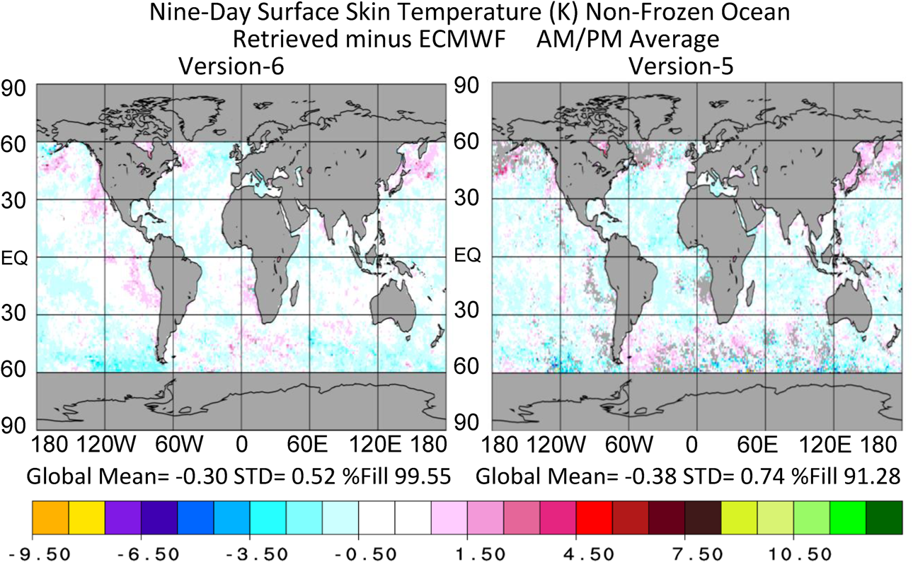 Figures 4(a) and 4(b) show the mean difference of the retrieved ocean surface emissivity from that of the AIRS science team ocean surface emissivity model as a function of satellite zenith angle for and , and Figs. 4(c) and 4(d) show the STDs of the retrieved values at a given zenith angle. The two channels shown are in the longwave and shortwave window regions, respectively. In these figures, we show statistics separately for a.m. orbits in dark colors and p.m. orbits in light colors. In both the longwave and shortwave window regions, version-6 (as well as version-6 AO) retrieved ocean spectral emissivities as a function of satellite zenith angle are very close to the values expected using the AIRS science team ocean surface emissivity model. Differences of version-6 retrieved values of from the ocean emissivity model are much smaller than those of version-5. Version-5 retrieved values of also showed a large spurious feature during the day in the vicinity of satellite zenith angle at both frequencies. This spurious feature occurs at the viewing angle at which maximum sunglint appears in the FOR. In addition to being more accurate in the mean sense, the retrieved values of are much more stable in version-6 compared to those of version-5, as evidenced by the much lower standard deviations of their values as shown in Figs. 4(c) and 4(d). There is no appreciable difference between version-6 and version-6 AO results related to retrieved ocean values of . Figures 4(a) and 4(b) show that daytime and nighttime version-6 retrieved values of ocean surface emissivity are not only close to those of the ocean emissivity model, which is a good measure of truth, but also very close to each other, as expected. Over land, surface spectral emissivity values change rapidly in space, and time as well, as a result of variations in ground cover, such as vegetation, rock, and soil types, and even snow cover. At a given location and day, these values should not change appreciably from day to night, however. Figure 5 shows the nine-day mean 1:30 a.m./1:30 p.m. differences of retrieved values of at 950 and over land obtained using the version-6 and version-5 retrieval systems. As in the case of ocean, day/night differences of version-6 retrieved land surface emissivity are much smaller than those of version-5, as they should be. 4.2.T(p) Retrieval Accuracy as a Function of YieldUnlike the major improvements made in version-6 methodology to retrieve surface skin parameters, the fundamentals of the methodology used in version-6 to retrieve temperature profile from AIRS cloud cleared radiances are basically the same as those used in version-5. Neverthless, version-6 temperature profile accuracy as a function of cloud cover is significantly improved over that of version-5 for a number of reasons. Foremost among these is the use of the Neural-Net temperature profile first guess, which is more accurate than the regression-based version-5 first guess, especially under more stressing cloud conditions. Version-6 retrieved temperature profiles also benefit from the improvement in version-6 surface skin parameters as well as improved version-6 QC methodology. Figure 6 shows statistics of the differences of QC’d version-5 and version-6 retrievals from collocated ECMWF truth for a global ensemble of cases taken over the nine focus days. Figure 6(a) shows the percentage of QC’d cases accepted as a function of height, Fig. 6(b) shows RMS differences of 1 km layer mean temperatures from collocated ECMWF truth, and Fig. 6(c) shows biases of QC’d 1 km layer mean differences from ECMWF. Statistics are shown for seven sets of results. We show in red the results for version-5 retrievals using three different QC procedures, in blue the results for version-6 retrievals using two different QC procedures, and in black the results for version-6 AO retrievals using QC procedures analogous to those of version-6. Fig. 6Global mean statistics of QC’d version-5, version-6, and version-6 AO temperature profiles, compared to ECMWF truth, using different QC thresholds. 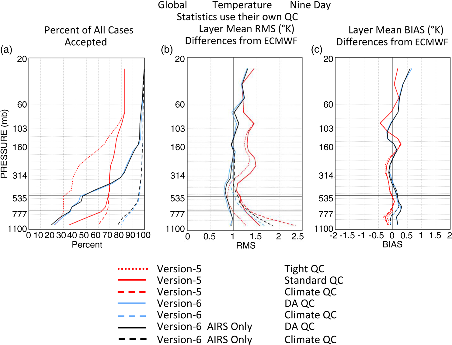 QC procedures used in both version-5 and version-6 designate two characteristic pressures for each temperature profile, and . These pressures are computed using thresholds of temperature profile error estimates . The Appendix describes the manner in which is computed and how it is used for QC purposes. Version-5 had only one set of QC error estimate thresholds, called standard thresholds, which were used to define version-5 values of , down to which retrievals were considered to be of highest quality. The version-5 standard thresholds were chosen such that if one utilized only retrievals down to for each case, this procedure would provide a middle ground of keeping retrievals with highest accuracy, which would be optimal for DA purposes on one hand, and keeping retrievals with the highest yield (best spatial coverage), optimal for climate purposes on the other hand. Experience using version-5 products showed that standard QC thresholds were optimal for neither purpose. For example, DA experiments assimilating version-5 retrievals down to a value of defined using a tighter set of thresholds than those of the official version-5 system, referred to as tight thresholds,12 resulted in significantly improved forecasts compared to assimilation of retrievals down to values of computed using the looser standard QC thresholds. The dotted red lines in Fig. 6 show acceptance yield and accuracy of version-5 retrievals down to as defined using the tight QC thresholds (not officially part of version-5). The solid red lines in Fig. 6 show equivalent statistics for the ensemble of version-5 retrievals down to as computed using the standard thresholds. The global yield of cases in which is equal to the surface pressure , as defined using standard thresholds, is shown in Fig. 6(a) to be . Utilization of an ensemble of retrievals with such a low yield would not be adequate for the generation of level-3 products with reasonable spatial coverage near the surface. The spatial coverage near the surface of such an ensemble of cases is particularly poor over land and sea-ice. In order to be able to generate level-3 products with reasonable spatial coverage in version-5, an additional case-by-case characteristic pressure, , was defined in an ad hoc manner over land and sea-ice for use in the generation of level-3 products. If was at least 300 mb over these domains, was set to be equal to the surface pressure . Otherwise, was set equal to . Version-5 level-3 products for at a given pressure were generated using all cases for which was . Over nonfrozen ocean, there was no need to include additional cases in the generation of a level-3 product with good spatial coverage, and over nonfrozen ocean was always set equal to . The dashed red lines in Fig. 6 show statistics for version-5 retrievals, which are included down to , i.e., statistics for the ensemble of cases used in the generation of the version-5 level-3 products. Global yield of version-5 cases down to at the surface has increased to , and the global mean RMS error of version-5 cases down to has increased to 2.7 K near the surface. Having learned from the experience with version-5 QC methodology based on the use of a single set of thresholds for both DA and climate applications, version-6 defines and independent of each other based on the use of two different sets of QC thresholds. A tight set of DA thresholds, optimized for DA purposes (cases with ), was used to derive , and a substantially looser set of climate thresholds, optimal for climate purposes (cases with ), was used to derive . The solid blue and black lines in Fig. 6 show statistics for version-6 and version-6 AO results, respectively, using their appropriate sets of DA QC thresholds, including all cases down to , and the blue and black dashed lines show results using the appropriate climate thresholds, including all cases down to . As in version-5, version-6, and version-6 AO, level-3 gridded products utilize all cases passing climate QC, that is, all cases down to . The Appendix provides detailed information about the QC methodologies used in version-5 and version-6, as well as the different thresholds used in each version. In version-5, all retrievals were either accepted or rejected above 70 mb based on the use of different types of tests, even before applying the error estimate based QC procedures.3 One of the tests that disqualified the entire temperature profile, and flagged the entire profile with (do not use), was that the retrieved cloud fraction is . Roughly 83% of version-5 retrievals passed the initial screening procedure, with none of them occurring under near overcast conditions. Version-5 retrievals with tight QC have considerably lower yield than those with standard QC below 200 mb, with correspondingly smaller RMS errors on the order of 1K beneath 300 mb. The ensemble of version-5 retrievals used to generate level-3 products (dashed red line) differs from that of those accepted down to . The yield near the surface is , which is better for the generation of level-3 products, but the RMS error for this larger ensemble of cases with or is much larger near the surface than those with . While RMS errors of retrievals increased with increasing yield, there is no appreciable difference in version-5 bias errors, compared to ECMWF, found using any of the three version-5 ensembles of cases shown in Fig. 6. Version-6 does not apply any test that eliminates the entire temperature profile, other than the requirement that the retrieval runs to completion. Version-6 retrievals using DA thresholds () have a yield much higher than those passing version-5 tight thresholds down to and have RMS errors at all levels, which has been found to be optimal for DA purposes.12 Among other benefits from the perspective of DA is that version-6 will allow for the assimilation of AIRS temperature products above the clouds, both in storms, as well as under overcast conditions in general. The yield of version-6 retrievals with climate QC (, 1) is extremely high throughout the atmosphere, with a value of at the surface. Achievement of this very high yield is extremely valuable in the generation of more representative version-6 level-3 products used for climate studies. RMS errors of version-6 retrievals with climate QC are better than, or comparable to, those of version-5 with standard QC down to the surface, and significantly better than that of the ensemble of version-5 retrievals used to generate level-3 products. Results for version-6 AO using either QC procedure are roughly comparable to those of version-6, but with slightly lower yields near the surface. The results shown in Fig. 6 are for all accepted retrievals, whether they were obtained during the night, when non-LTE and reflected solar radiation do not affect shortwave radiances, or during the day, when these effects must be well accounted for in order to produce accurate retrievals. Figure 7 is analogous to Fig. 6, but breaks down the version-6 results shown into those obtained during the night (1:30 a.m.) and those obtained during the day (1:30 p.m.). Figure 7 shows that there is essentially no difference in the quality of the results obtained at night and those during the day. This implies that effects of non-LTE on shortwave radiances during the day are well accounted for by the AIRS RTA. This result also implies that cloud cleared radiances obtained during the day are as accurate as those obtained at night and, indeed, that the procedure used to generate cloud cleared radiances also accounts for the effects of solar radiation reflected by clouds in the AIRS FOVs. Fig. 7Global nine-day version-6 temperature profile statistics shown separately for daytime and nighttime cases. 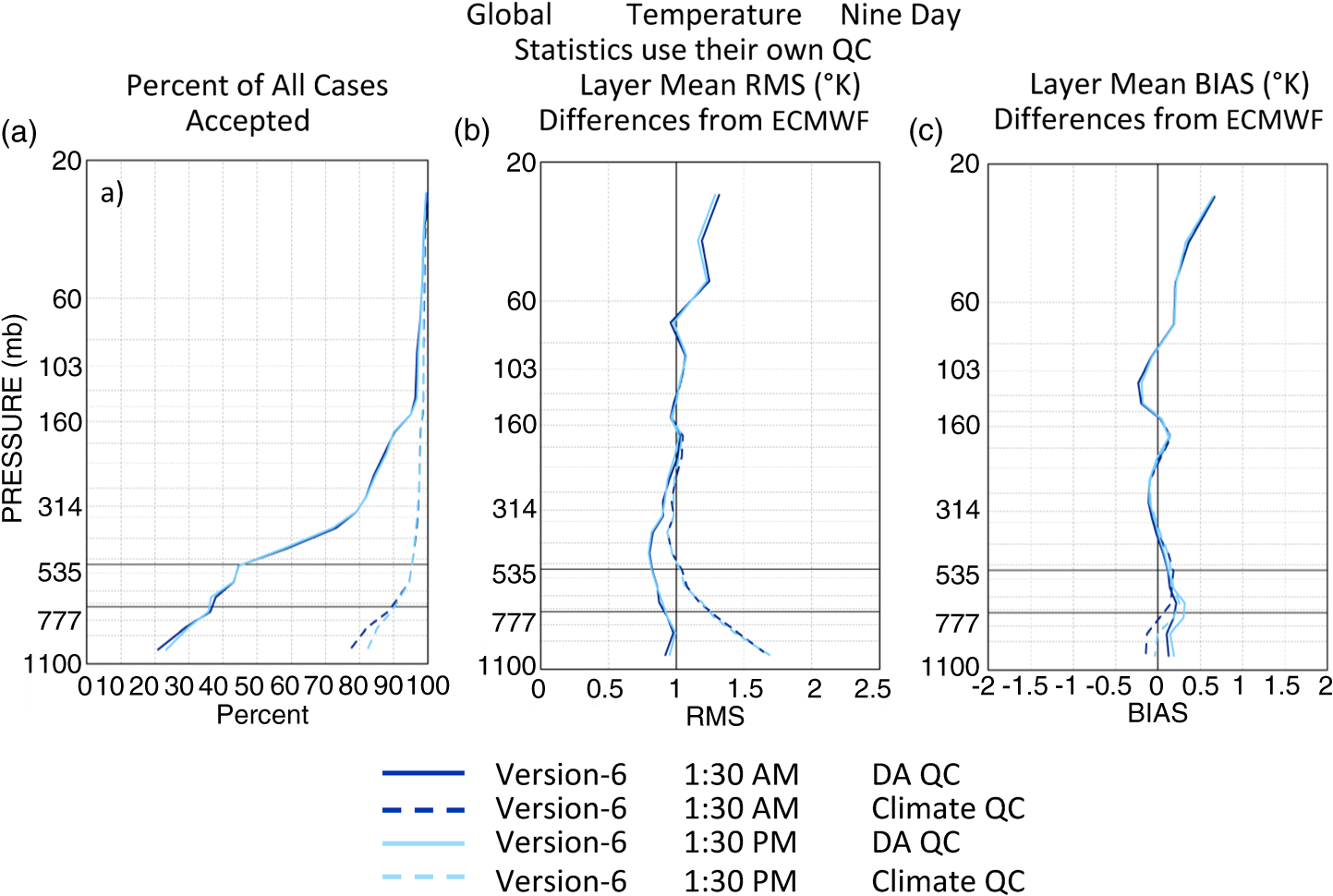 Figures 8(a) and 8(b) compare RMS errors of QC’d version-6 and version-5 retrievals with those of their first guesses. The solid and dashed blue and red lines shown in Fig. 8 are identical to those in Fig. 6(b). The RMS errors of the first guesses are shown by light blue lines for version-6 and pink lines for version-5. Figure 8(a) shows that the version-6 retrievals improve on the Neural-Net guess at all pressures , especially for the easier ensemble of cases accepted using DA thresholds. Version-6 retrievals are slightly poorer than their first guess above 60 mb, which is at least in part due to the fact that the Neural-Net guess above 60 mb is extremely accurate. Figure 8(b) shows that essentially the same relative result holds for version-5, though in version-5 the retrievals always improve on their first guess, which is less accurate than the Neural-Net, at all levels. In addition, unlike for version-6, the improvement over the first guess is greatest in the mid-troposphere. Fig. 8Comparison of the accuracies of QC’d version-6 and version-5 retrieved temperature profiles with those of their initial guesses. 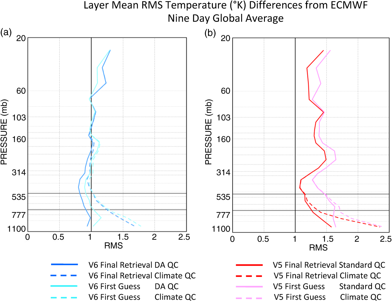 4.2.1.T(p) retrieved accuracy as a function of cloud fractionFigure 9(a) shows % yields of version-5 and version-6 retrievals, accepted using version-5 standard QC and version-6 climate QC, respectively, as a function of retrieved cloud fraction at three mid-lower tropospheric pressures, and Fig. 9(b) shows the RMS errors over three corresponding 1-km layers. Version-6 climate QC yields are much higher than those of version-5 at all cloud fractions, especially at larger cloud fractions. Version-6 RMS errors over these larger ensembles of cases for all cloud fractions are also considerably better than those of the smaller version-5 ensembles. The fact that version-6 retrievals remain accurate and improve over the Neural-Net first guess at larger cloud fractions indicates that the version-6 cloud cleared radiances are accurate as well under more difficult cloud conditions. Fig. 9(a) Percent acceptance, using climate QC, of global version-5 and version-6 temperature profiles as a function of retrieved fractional cloud cover at three select pressure levels. (b) RMS difference of version-5 and version-6 1 km layer mean temperatures from colocated truth in three select layers.  4.3.Retrieval Accuracy of q(p)The details of the retrieval step are essentially unchanged from what was done in the retrieval step both in version-5 and in version-4. Version-7 will address further improvements to be made to the retrieval algorithm. Nevertheless, version-6 retrieved values of are improved over those of version-5 as a result of the same factors that led to improved version-6 values of as compared to version-5: (1) improved surface skin temperatures and spectral emissivities, (2) an improved first guess provided by the Neural-Net start-up system, and (3) improved clear column radiances . Version-6 retrieved values of also benefit from improved values of that are used as input to the retrieval step. Figure 10 shows results analogous to those of Fig. 6 comparing QC’d 1-km layer precipitable water to that of collocated values of ECMWF. We show results only up to 200 mb, above which water vapor retrievals are considered to be of minimal validity and are not included in the AIRS science team standard product data set. The relative results comparing version-5 and version-6 retrievals are analogous to those found for . Version-6 retrievals with both DA and climate QC are considerably improved over those of version-5 in the lower troposphere. This improvement in the lower troposphere is at least partially a result of the improved values of and in version-6 compared to version-5. As with , version-6 retrievals with climate QC are unbiased, have high accuracy, and contain almost complete spatial coverage. Globally, version-6 AO retrievals are slightly less accurate than those of version-6 near the surface. This difference between results of version-6 and version-6 AO occurs primarily over the ocean and is a result of the benefit over ocean of the 22- and 31-GHz channels of AMSU-A, which are not included in the AIRS only retrieval procedure. Fig. 10Global mean statistics of QC’d version-5, version-6, and version-6 AO water vapor profiles, compared to ECMWF truth, using different QC thresholds.  In version-6, is flagged to be of highest quality () if the water vapor profile has best quality () down to the surface and is flagged to be of good quality () if the water vapor profile has good quality () at the surface. This same test is also applied to generate QC flags for (1) surface air temperature, (2) clear sky OLR, (3) , , and CO profiles, and (4) surface skin temperatures over land and nonfrozen ocean. Figure 11 shows the spatial distribution of the pseudo-level-3 nine-day mean field of accepted cases of total precipitable water, , flagged to be of climate quality (, 1). The statistics shown for version-6 and version-5 represent the % of grid points containing values, the area weighted global mean difference of the gridded level-3 values of from the collocated ECMWF values of , and the area weighted spatial standard deviation of those values from ECMWF. Statistically, the version-6 pseudo nine-day mean level-3 values of are considerably more accurate than those of version-5, especially over land. This improvement of is partially a result of improved version-6 surface skin parameters, especially over land. Version-5 used a different procedure to accept those values of to be used in the generation of the level-3 product than that used in version-6. 4.4.Yield Trends and Spurious Bias Trends of T(p)Our research using version-5 retrieved products indicated that QC’d version-5 values of had a large negative yield trend, as well as spurious bias trends when compared to collocated ECMWF values of . A prime consideration in the finalization of version-6 was to alleviate these negative yield trends and spurious bias trends as much as possible. Figure 12 shows yield trends and temperature bias trends of version-5 retrievals using standard QC, and both version-6 and version-6 AO retrievals using climate QC, as evaluated over the nine days used in all other figures. Figure 12(a) shows that the % yield of accepted version-5 retrievals was decreasing over time (negative yield trend), and Fig. 12(b) shows that version-5 retrievals had substantial negative spurious temperature bias trends in the troposphere, which were in part due to the fact that the regression first guess used in version-5 had a negative tropospheric temperature bias trend itself. A substantial part of the negative yield trend was due to a significant degradation of the noise characteristics of AMSU-5. Version-6 contains modifications that alleviated these problems, one of which is that version-6 no longer uses AMSU-5 at all. Other factors also contributed to the spurious temperature bias trends found in version-5, and these were also corrected in version-6. Fig. 12Global mean yield and spurious layer mean temperature bias trends of QC’d version-5, version-6, and version-6 AO retrievals as a function of pressure.  Figure 12 shows that version-6 has eliminated the substantial negative tropospheric temperature profile yield trends, on the order of 2% per year, which were found in version-5. In addition, the version-6 negative bias trends beneath 500 mb are much smaller than those of version-5, which were as large as . Part of this improvement is due to the fact that the Neural-Net first guess used in version-6 does not appear to have any spurious trends associated with it. In addition, version-6 does not use any channels sensitive to in the retrieval step, which were used in version-5. These channels are no longer used in the temperature profile retrieval step because the concentration of has been changing over time and this is not accounted for in the AIRS RTA. There is no appreciable difference between the yield or bias trend results obtained for version-6 and version-6 AO. 4.5.Comparison of Version-6 and Version-5 Retrieved Values of Cloud Fraction and Cloud Top4.5.1.PressureThe procedure used to derive cloud fraction and cloud top pressure in version-6 is similar to that used in version-5,1,3 but version-6 has a number of significant improvements. The radiatively effective cloud fraction at frequency , is given by the product of , the geometric fractional cloud cover of an AIRS FOV as seen from above, and , the cloud spectral emissivity. The AIRS science team cloud parameter retrieval methodology determines only the product of these two terms, , along with a corresponding cloud top pressure , for each of up to two layers of clouds in a given scene.1,3 A basic simplifying assumption of the cloud retrieval methodology used in both version-5 and version-6 is that the clouds are gray, that is, is independent of frequency. Version-5 simultaneously derived 20 parameters for each AIRS FOR, nine effective cloud fractions and , one pair for each AIRS FOV contained within the AMSU FOR, along with two cloud top pressures , and considered to be representative of the pressures of each of the two layers of clouds covering the entire AIRS FOR. In version-6, the cloud parameter retrieval step is performed separately for each AIRS FOV to determine the four parameters, , , , and , in each FOV. A total radiatively effective cloud fraction for the entire FOR, , is computed as the average cloud fraction according to and an effective cloud top pressure for the entire FOR is computed as the weighted average of all nine values of and in the FOR as was also done in version-5. The version-6 level-2 product contains individual values of , , , for each AIRS FOV, as well as the single FOR heritage values and defined according to Eqs. (4) and (5).Cloud parameters in an AIRS FOV are derived such that channel radiances computed using these cloud parameters , where is a state vector for the FOV, best match the observed radiances in that FOV for the ensemble of cloud retrieval channels . The channels used to determine cloud fraction and cloud top pressure are the same as those used in the cloud clearing step and are shown by yellow stars in Fig. 1. The state vector used to derive cloud parameters in an AIRS FOV is the geophysical state retrieved for the entire AIRS FOR containing the nine FOVs. In version-5, the state vector used to derive values of and in an FOR was the retrieved state used in the final cloud clearing step for those cases in which a successful combined AIRS/AMSU retrieval was performed. In the roughly 27% of the cases in which the AIRS/AMSU retrieval was rejected (see Fig. 6), the state used to derive cloud parameters was the so-called fallback state that was obtained from a previously performed AMSU only retrieval step.3 Cloud parameters retrieved using the fallback state vector were flagged as , and those retrieved using the final retrieval state vector were flagged as . Under some conditions, the cloud parameter retrieval step was not able to complete successfully, and clouds retrieved for those cases were flagged as in version-5. In version-6 and version 6 AO, successful retrievals are performed under essentially all conditions, and there is no need to use derived from a microwave fallback state. Nevertheless, version-6 does resort to the use of derived from a partial fallback state under some circumstances in which part of the retrieved state is known to be of poor quality and a better alternative is available. In particular, values of retrieved under either near overcast or overcast conditions over ocean can be spuriously very low. These values of will, in general, be flagged as bad, with , meaning they are not used in the generation of the level-3 product. Associated values of retrieved under these conditions will also be poor and are also flagged to be of poor quality. Nevertheless, some value for and must be included in the state vector used to derive the cloud product. We have found that the initial guess coming from the Neural-Net start-up procedure gives reasonable values over nonfrozen ocean even for very cloudy cases. Therefore, over ocean, if , we assume the retrieved values and are in error and replace and in the retrieved state vector by and while retaining the remainder of the retrieved state vector when computing cloud parameters. We have found that Neural-Net values of over land or ice are not of sufficiently good quality for use in the generation of cloud parameters, so this test and replacement procedure is done only over open ocean. As in version-5, cloud parameters retrieved in such fallback cases are flagged as . Cloud parameters retrieved under almost all other cases, which represent the vast majority of the cases, are flagged as . Under the extremely rare conditions in which the final cloud parameter retrieval step does not complete successfully, cloud parameters are flagged as as was done in version-5 and are not used in the generation of the level-3 cloud products. A complication in the cloud parameter retrieval methodology is that the best least squares fit may result from a cloud parameter solution that lies in a region that is unphysical. To avoid an unphysical result, we do not allow retrieved cloud fractions to be or ; nor do we allow cloud top pressures to be very close to the surface or above the tropopause. Because of the way these constraints were handled in version-5, many cloud retrievals in version-5 failed to converge properly. We made numerous enhancements in version-6, which stabilized the cloud parameter retrieval step and also allowed for cloud top pressures to lie closer to the surface than was allowed in version-5. Figure 13(a) shows the number of cases in which a nonzero cloud fraction was retrieved as a function of cloud top pressure for version-5, version-6, and also for version-6 AO. Two features are readily apparent from Fig. 13(a): the distributions of the number of cases obtained as a function of retrieved cloud top pressure are essentially identical in version-6 and version-6 AO, and both are substantially different from that of version-5. Version-5 has spikes in the number of cases retrieved at select pressures, such as 200, 300, 350, 750, 850, and 950 mb, which resulted from the cloud retrieval algorithm’s inability to converge properly in those cases. Such features are not observed in either version-6 or version-6 AO. Even more significant is the shift to higher pressures in the peak of the occurrence of low clouds in version-6 as compared to version-5. This difference near 1000 mb is, in part, due to the constraint used in version-5 that must be at least 50 mb above the surface, while in version-6, was allowed to go down to 10 mb above the surface. The large shift in the peak in the number of clouds retrieved in version-5 as a function of cloud top pressure, from to in version-6, is a combined result of changes not only in the cloud parameter retrieval step, but also in the state vector used in version-5 compared to that used in version-6, which does not use a microwave only fallback retrieval state. Fig. 13Global statistics of version-5, version-6, and version-6 AO cloud parameter retrievals as a function of retrieved cloud top pressure: (a) Number of retrieved cases for a given cloud top pressure. (b) Average retrieved cloud fraction of a function of cloud top pressure.  Figure 13(b) shows plots analogous to those shown in Fig. 13(a), but shows the average cloud fraction found for each cloud top pressure . Cloud fractions in version-6 and version-6 AO are again very close to each other and differ significantly at some cloud top pressures from those of version-5. Version-6 has more clouds than version-5, between 130 and 400 mb. On the other hand, version-6 has fewer clouds than version-5, between and 750 mb, which corresponds to the pressure interval in which the maximum numbers of cloud parameter retrievals occurred in version-5. Figure 13(b) shows spikes in the retrieved cloud fraction in version-5 at the same pressures in which they occurred in Fig. 13(a). These version-5 spikes in Fig. 13(b) are negative at pressures , indicative of the fact that the spurious cloud retrievals occurring at these discrete pressures had low, probably , cloud fractions. On the other hand, these spikes in Fig. 13(b) for version-5 were positive at pressures 700 mb and greater, indicative that these spurious cases had large cloud fractions, most likely close to 100%. Version-5 also had a somewhat disconcerting peak near 90 mb in Fig. 13(b), but Fig. 13(a) shows that there were very few such cases. Figure 14 shows the spatial distributions of values of cloud fraction and cloud top pressure for the daytime and nighttime orbits on August 10, 2007 as retrieved using version-5 and version-6. These plots depict both and at the same time. There are seven different color scales used for different intervals of , as indicated on the figures. Reds, violets, and purples indicate high (low pressure) clouds, blues and greens indicate mid-level clouds, and oranges and yellows indicate low clouds. Within each color scale, darker colors indicate greater fractional cloud cover, and paler colors indicate lower fractional cloud cover. While the basic cloud patterns are the same in version-6 and version-5, the cloud features are much more coherent, and the colors are darker, in version-6. Of particular significance are the coherent areas of dark orange, depicting extensive cloud cover with cloud top pressures between 680 and 800 mb, found in version-6 that are at best muted in version-5. This finding is indicative of the better ability to derive the existence of stratus clouds over ocean in version-6 as compared to version-5. Particularly noteworthy is the region in the vicinity of 30°N, 120°W, off the West Coast of North America, in which version-6 depicts extensive stratus cloud cover at both 1:30 a.m. and 1:30 p.m., while version-5 shows very little cloud cover at all. The results shown in Fig. 13(a) are suggestive of this result because many more cases with exist in version-6 as compared to version-5. Another noteworthy improvement in version-6 clouds compared to version-5 is that the spatial distribution of clouds in version-5 has many missing grid points in which no successful cloud retrieval was performed. Fig. 14Version-6 and version-5 retrieved cloud fractions and cloud top pressures for 1:30 a.m. and 1:30 p.m. orbits on August 10, 2007. 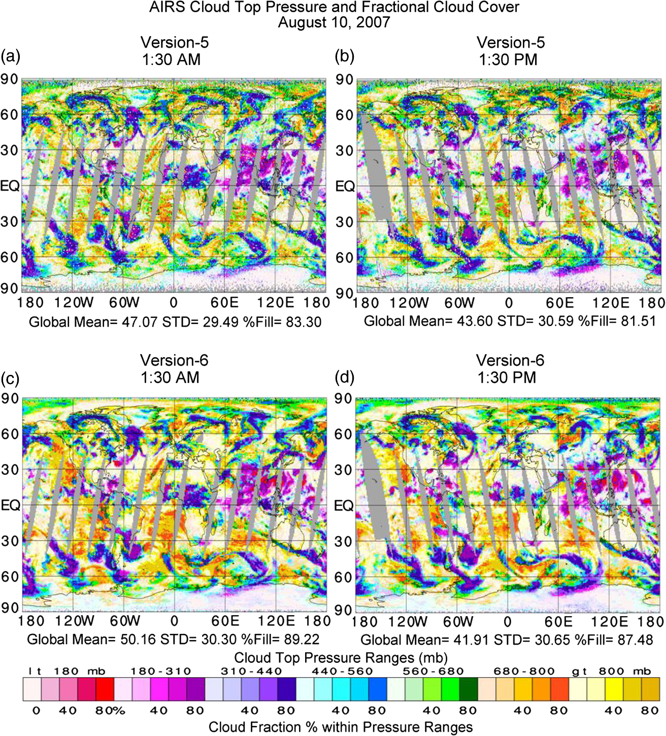 There are very few missing grid points (other than orbit gaps) found in version-6. The percent of grid boxes in which data exist, indicated beneath each figure, shows that version-6 has retrieved cloud parameter values in more of the grid boxes than does version-5, both at 1:30 a.m. and 1:30 p.m. Kahn et al.13 give more details about the updates to the cloud parameter retrieval algorithm in version-6 as compared to version-5 and show that the higher spatial resolution cloud top pressures, and corresponding cloud top temperatures found in version-6, have coherent spatial structure and contain a larger range of values than is found in version-5. Kahn et al.13 also show a much better agreement of retrieved version-6 cloud parameters, as compared to version-5, with those found in CloudSat and CALIOP data. Kahn et al.13 also introduce the new version-6 products of cloud thermodynamic phase, ice cloud effective diameter, and ice cloud optical thickness, which are derived on an AIRS FOV basis using other AIRS retrieved products as a starting point for their radiative transfer calculations. 4.6.Outgoing Longwave RadiationAIRS OLR is computed for each AIRS FOV in which a successful cloud parameter retrieval is performed. QC flags used for OLR are identical to those used for cloud parameters. OLR is computed via a radiative transfer calculation, which generates the total longwave flux to space expected for the final retrieved state vector , including the retrieved cloud parameters. More details of the methodology used to calculate AIRS version-5 and version-6 OLR are given in Susskind et al.14 Susskind et al.14 show that version-5 OLR gives good agreement with CERES OLR, in terms of both absolute values and anomaly time series on a latitude-longitude spatial scale. Susskind et al.14 also show that version-6 OLR gives even better agreement with CERES than does version-5 OLR. Part of this improvement of OLR in version-6 is a result of the improved accuracy of version-6 retrieved products as compared to version-5. In addition, version-6 uses an improved OLR radiative transfer parameterization15 compared to what was used in version-5.16 5.Quality Controlled Values of Clear Column RadiancesThe clear column radiance for channel , , is a derived quantity and, like other version-6 derived quantities, has case-by-case, channel-by-channel, error estimates , generated in a manner that is described in the Appendix. Version-6 and version-6 AO use thresholds of to generate case-by-case, channel-by-channel, QC flags for , in a manner described in the Appendix. Channel-by-channel QC flags were not a feature of version-5. Figure 15 shows statistics over the spectral interval from 650 to , related to QC’d values of for all oceanic cases within the latitude band of 50°N to 50°S generated using the nine-day ensemble of retrievals. The top panel of Fig. 15 shows the percent of all cases, as a function of frequency, passing loose climate thresholds (, 1), and tight DA thresholds (), in light and dark colors, respectively. Results are shown in shades of blue for version-6 and in shades of black for version-6 AO. Percent yields are greater for cases passing the climate QC test as compared to the DA QC test, as expected, but it is important to note that there are no appreciable yield differences between version-6 and version-6 AO QC’d values of with regard to either test. The second panel of Fig. 15 shows the mean values of over all cases with , where is the clear column brightness temperature given by the blackbody temperature corresponding to . is indicative of the temperature of the portion of the atmosphere to which the channel is most sensitive. Channels with are sensitive primarily to stratospheric temperatures, and among such channels, those with larger values of sound higher in the stratosphere. The reverse is true for channels with , which are sensitive primarily to tropospheric temperatures, and in which higher values of indicate increased sensitivity to temperatures in the lower portions of the troposphere, and eventually to the surface skin temperature. Yields of QC’d values of generally decrease with increased channel sensitivity to lower tropospheric and, eventually, to surface skin temperatures. Figure 15 shows that yields of accepted values of using DA QC thresholds are 50% or higher for channels up to , which have considerable sensitivity to surface temperature. Yields are higher for those channels sensing higher in the atmosphere, in which observed radiances are less sensitive to cloud cover and are, therefore, less sensitive to cloud clearing errors. Fig. 15Statistics for QC’d version-6 and version-6 AO cloud cleared brightness temperatures over the spectral interval from 650 to , using two sets of QC thresholds. Results shown are for all accepted oceanic cases 50°N to 50°S.  The third panel of Fig. 15 shows the STDs of QC’d values of referred to as , and also shows in yellow the mean values of the equivalent brightness temperature channel noise , given by the single FOV channel radiance noise evaluated at . Values of are computed on a case-by-case basis using the collocated ECMWF state in conjunction with the AIRS RTA. Errors in both the state and in the AIRS OLR forward calculation will each contribute to errors in . Over land, the surface parameters and used for truth both contain considerable uncertainty, and they contain some uncertainty over ocean as well. The results shown in Fig. 15 are for ocean cases only because we do not have accurate estimates of over land for channels sensitive to the surface. Errors in arise from two sources: instrumental noise and cloud clearing errors, as discussed in detail in Appendix. The channel clear column radiance is obtained as a linear combination of the observed radiances for that channel in each of the FOVs used to generate the retrieval.3 For channels thought to be unaffected by clouds, the nine observations are averaged together, and this averaging results in a multiplicative channel noise reduction factor of for channels that do not see clouds. Consequently, the STDs of for stratospheric sounding channels are actually lower than the instrumental noise, especially using DA QC as shown in the darker colors. In general, the taking of a linear combination of to obtain amplifies the effect of channel noise on , especially in the case of more difficult cloud cases.3 Therefore, even if the coefficients used to determine from were perfect, the STD of would exceed for channels sensitive to clouds in the FOR. The largest potential source of errors in results from errors in the cloud clearing coefficients used to derive . For both these reasons, the STD of increases as frequencies become more sensitive to lower tropospheric and surface temperatures and whose radiances are more greatly affected by clouds. Part of the errors shown at higher is an artifact resulting from the effect of the uncertainty in ocean surface skin temperature and ocean spectral emissivity on the values of in channels sensitive to the surface. In any event, the STDs of using DA QC are not appreciably larger than channel noise up to . The fourth panel of Fig. 15 shows biases of . Biases of for all four ensembles of cases are similar to each other. The small biases outside the higher frequency window region are partially a result of biases in rather than in , as well as a result of systematic errors in the RTA. The negative bias of in channels more sensitive to the surface may be real and be the result of insufficient cloud clearing when very low clouds are present. The most important potential application of using QC’d values of is with regard to DA. ECMWF and National Centers for Environmental Prediction (NCEP) assimilate observed AIRS radiances operationally. In particular, ECMWF and NCEP assimilate AIRS radiances primarily in the spectral interval of to . These channels are assimilated on a case-by-case, channel-by-channel basis, using radiances only in those channels whose observed radiances are thought to be unaffected by clouds. In principle, operational centers could assimilate values of in an analogous way given appropriate error estimates and QC procedures. The spatial coverage of DA QC’d is significantly greater than that of radiances unaffected by clouds, especially for tropospheric sounding channels. Figure 15 shows that values of with over ocean for the most part have yields of 70% or better at frequencies . Moreover, the STD of the errors in with are on the order of the channel noise at these frequencies. For those cases in which the errors in are greater than the channel noise, their individual errors are characterized very well by and this can be taken into account by the DA procedure. 6.SummaryAIRS/AMSU observations are now being processed near real time at the Goddard DISC using both the AIRS science team version-6 retrieval algorithm as well as the AIRS only processing system version-6 AO, which does not use AMSU observations in any way. All AIRS data since September 2002 has been reprocessed using both algorithms. Results using AIRS version-6 AO are almost as good as those obtained using AIRS version-6, and both are significantly better in every way than those obtained previously using the AIRS science team version-5 algorithm. The success of version-6 AO is extremely important for two different reasons. The most immediate reason is that it serves as an important backup processing mode for AIRS data in the event that the AMSU instrument, which has been degrading over time, further degrades significantly. The AIRS instrument is showing essentially no signs of degradation and is expected to generate good data as long as the Aqua spacecraft remains in a stable orbit, perhaps until 2022 or even later. In addition, this result demonstrates that while desirable, it is not essential for future atmospheric sounding missions carrying a high spectral resolution IR sounder, such as on a geostationary sounder or on low Earth orbit CubeSats, to carry a microwave sounding instrument to accompany the advanced IR sounder. The AIRS science team version-6 retrieval algorithm contains a number of significant advances over what was done in version-5. The most important advance is that the physical retrieval methodology used in version-6 determines information about surface skin temperature using cloud cleared radiances only in the shortwave window region of 2396 and , while version-5 determined surface skin temperature using cloud cleared radiances in shortwave window channels simultaneously with those in the longwave window region. This modification resulted in a significant improvement in the quality of both ocean and land surface skin parameters retrieved in version-6, compared to version-5, during both daytime and nighttime conditions. In the past, there had been a reluctance to use shortwave window observations for retrieval purposes because shortwave channels are affected significantly by solar radiation reflected both by clouds and the surface. Neither phenomenon is a problem for the version-6 retrievals, however. The cloud clearing procedure accounts well for solar radiation reflected by clouds, and the determination of the surface spectral bidirectional reflectance as part of the surface parameter retrieval step accounts well for solar radiation reflected by the surface. As in version-5, tropospheric temperatures are determined using only shortwave channels in the vicinity of . The version-6 temperature profile retrieval algorithm is in most aspects similar to that used in version-5. The main improvement lies in the use of a Neural-Net generated first guess in place of the regression-based first guess used in version-5. The Neural-Net first guess is, in general, more accurate than the regression guess, but it is especially so under more stressing cloud conditions. This is the main reason that version-6 produces accurate QC’d temperature profiles under much more stressing cloud conditions than those obtained in version-5. Version-6 temperature profiles also benefit from improved values of surface skin temperature and surface spectral emissivity. There has been no change in the water vapor profile retrieval algorithm between version-5 and version-6, but version-6 water vapor profiles are also improved over those of version-5 as a result of improvements in the determination of other geophysical parameters, as well as the resulting improvements in cloud cleared radiances, especially under more extensive cloud cover. Version-6 cloud products are also significantly improved over those of version-5 both because of improvements in details of the cloud parameter retrieval methodology and also the benefit of more accurate retrievals of other geophysical parameters under more stressing cloud cover conditions. Finally, version-6 OLR is improved over version-5 both because of better values of all other retrieved parameters, as well as the use of an improved OLR RTA15 in version-6. The error estimate methodology used in version-6 is similar to that used in version-5, but there has been a significant improvement in the use of error estimates for QC purposes, especially for climate QC purposes. Version-6 climate QC takes advantage of the ability to generate accurate retrievals under almost all cloud conditions, and version-6 level-3 products now include accurate retrievals with almost complete spatial coverage, even down to the surface. All AIRS version-6 and version-6 AO level-2 and level-3 products can be obtained at the Goddard DISC http://disc.sci.gsfc.nasa.gov/AIRS/data-holdings. Spot-by-spot level-2 products are available on an AIRS FOV basis, and gridded level-3 products are presented on a latitude-longitude grid, gridded separately for 1:30 a.m. orbits and 1:30 p.m. orbits, on a daily, eight-day mean, and monthly mean basis. More details are given in Olsen et al.17 and Manning et al.18 AppendicesAppendix:Error Estimates and Quality Control ProceduresA.1.IntroductionEach retrieved quantity in version-5 and version-6 has an associated error estimate . A major advancement in version-5 was the development of a methodology to generate accurate empirical error estimates for a number of geophysical parameters and to use thresholds of these error estimates for quality control (QC) purposes. Analogous procedures are also used in version-6, with some improvements in the details. Version-4 (Ref. 2) used threshold values of 12 internal tests for the purpose of generating QC flags for different geophysical parameters. Version-5 (Ref. 3) used the case-by-case values of these 12 internal tests, as well as values of four additional tests, as predictors to generate empirical case-by-case error estimates for select geophysical parameters . Version-6 uses a methodology analogous to that used in version-5 to generate empirical error estimates , with some modifications resulting from changes in the steps used in the version-6 retrieval system as compared to those used in version-5. A.1.1.Generation of the empirical error estimates Ts, T(p), and WTOTVersion-5 used case-by-case values of 16 internal tests as predictors in the generation of the empirical error estimates , , and for case . Appendix B of Susskind et al.3 gives a description of the meaning of these 16 tests. The symbols used for these tests, including their superscripts, have version-5 heritage, and we maintain the use of the same symbols in the description of the tests used in version-6. Some of these tests involve procedures used to generate the start-up state used as the initial guess for the physical retrieval sequence of steps. is also used in the generation of the first pass clear column radiances , which are the input to the first phase of the physical retrieval process. The sequences of steps used to generate in version-5 and version-6 differ from one another. For this reason, the relevant tests used in each retrieval system are analogous to each other, but refer to results obtained using different states. In version-5 and version-6, and are both computed according to where is the error estimate of retrieved geophysical parameter for case , is the value of the ’th predictor for case , is a matrix, and is the number of predictors used to determine the error estimates. Error estimates are by definition all positive. Values of the predictors are also all positive, and in general, larger values of are indicative that a poorer retrieval will be obtained for case .The meanings and significance of the 16 predictors used in Eq. (6) in version-5 were as follows: (1) is the final retrieved effective cloud fraction (%); (2) is the integral cloud liquid water () retrieved as part of a start-up advanced microwave sounding unit (AMSU) only retrieval step; (3) represents the difference between the retrieved lower-tropospheric temperature obtained in a test microwave only retrieval step and that determined in the final physical retrieval step (K); (4) is the channel noise amplification factor obtained in the cloud clearing step, which generates (unitless); (5) is the effective channel noise amplification factor obtained in the final cloud clearing step that generates , which are the values of clear-column radiances used in the second pass physical retrieval sequence of steps (unitless); (6) represents the quality of the cloud clearing fit obtained in a start-up cloud clearing step used to generate (unitless); (7) represents the degree to which the final physical temperature profile retrieval step has converged (unitless); (8) represents the degree to which the final physical surface parameter retrieval step has converged (unitless); (9) represents the effective channel noise amplification factor resulting from the cloud clearing step used to generate (unitless); (10) represents the agreement between the observed AMSU channel 5 brightness temperature and that computed from the solution obtained in the final physical retrieval step (K); (11) represents the difference between the final retrieved value of and the value of contained in the start-up state (K), which is generated in version-5 by a clear regression step; (12) represents the principal component reconstruction score of the observed atmospheric infrared sounder (AIRS) radiances that is obtained as part of the start-up clear regression step (unitless); (13) represents the difference between the final retrieved value of and that contained in (K), which is generated by a cloudy regression step; (14) represents the difference between the retrieved lower-tropospheric temperature of the final state and that contained in ; (15) represents the degree of convergence of the physical retrieval water vapor retrieval step (unitless); and (16) represents the degree of convergence of the cloud clearing step used to generate (unitless). In version-6, neither a cloudy regression step nor a clear regression step is used as part of the start-up procedure. These two steps are replaced in version-6 by a single Neural-Net start-up step that generates . The state used as the initial guess to the physical retrieval process is generated in version-6 by using as input to an AMSU only retrieval step, which modifies so as to give . In version-6 AIRS only (AO), the AMSU only retrieval step is not performed and is given by . The error estimate predictors used in version-6 are basically the same as those used in version-5 with three exceptions: (1) Predictor 10 used in version-5 was the difference between the observed brightness temperature in AMSU-A channel 5 and the brightness temperature for that channel computed using the final retrieved state. AMSU-A channel 5 has degraded significantly and is no longer used in any way in the version-6 retrieval process. An analogous predictor is now used in version-6 involving AMSU-A channel 6. This changes the data used for one predictor, now called , in version-6. (2) Predictor 12 used in version-5 related to how well the National Oceanic and Atmospheric Administration (NOAA) clear regression step performed. The NOAA clear regression step is not performed in version-6, and predictor 12 is not computed and, therefore, not used in the generation of error estimates in version-6. This eliminates one predictor used in version-6 from those used in version-5. (3) Predictors 11 and 13 used in version-5 related to the differences between the retrieved surface skin temperature and the skin temperatures obtained using each of the clear and cloudy regression steps in version-5. In the Neural-Net start-up system, there is only one value of surface skin temperature used in the start-up procedure. Therefore, only a single test of this type, given by the difference between the retrieved value of and the value of found in , is used as a predictor in the generation of error estimates in version-6. This eliminates one additional predictor in version-6 compared to what was used in version-5. Consequently, version-6 uses only 14 error estimate predictors in Eq. (6). Version-6 predictors 2, 3, and 10 all involve use of AMSU-A observations in one manner or another and are not used in the version-6 AO retrieval system. Consequently, version-6 AO uses 11 predictors in the generation of . Finally, it has been determined that while the Neural-Net values of are very accurate over ocean, they are not sufficiently accurate over land or frozen ocean for use as an error estimate predictor. Consequently, over land and frozen ocean, the predictor involving the difference between retrieved and Neural-Net surface skin temperature is not used in version-6. Therefore, over land or sea ice, only 13 predictors are used in version-6 and 10 predictors are used in version-6 AO. The coefficients of are determined in essentially the same manner in version-6 as was done in version-5. In version-6, we generate six distinct matrices for separate use under daytime or nighttime conditions, as well as for separate use over (1) non-frozen ocean, (2) nonfrozen land, and (3) frozen (ice or snow) cases. In version-5, only four such matrices were used, in which a single pair of matrices (day and night) was used to be representative of all cases in categories 2 and 3, and a separate pair of matrices was used over nonfrozen ocean. The coefficients of the matrix for an ensemble of cases can be determined in a straightforward manner if one is given the true values of , . is determined by finding the coefficients that minimize the RMS difference of , where , and when is used in Eq. (6) to generate . The coefficients of are determined separately for each parameter . In order to generate the version-6 coefficients for each of the six different matrices , we used appropriate spatial subsets of and , generated using all version-6 retrievals that were performed on September 29, 2004 and February 24, 2007, along with the collocated ECMWF 3-h forecast values of as . The coefficients of the six sets of matrices were determined separately for version-6 and for version-6 AO based on observations on these two days and are then used for all time periods. In both version-5 and version-6, the error estimate for total precipitable water is computed in a manner analogous to that used to compute and , but is computed in terms of the fractional error estimate. where FE is the fractional error in total precipitable water. The predictors used in Eq. (7) are identical to those used in Eq. (6). The error estimate for is obtained according to . The value of total precipitable water used in Eq. (7) is not derived directly in the physical retrieval, but is computed as the vertical integral . The coefficients of are determined in a way otherwise analogous to those of , but by minimizing the RMS difference of when is used in Eq. (7).A.1.1.1.Nonfrozen ocean surface skin temperature quality controlVersion-5, version-6, and version-6 AO all use the nonfrozen ocean skin temperature error estimate directly for QC, with separate thresholds and used to indicate best quality retrievals for which , which are flagged as , and good quality retrievals, where , which are flagged as . Cases with either or are those used in the generation of the level-3 product over ocean. Cases with are flagged as having poor quality with . QC flags defined in this manner are what were used in the generation of the results shown in Fig. 2. Values of these thresholds are shown in Table 1 for version-5, version-6, and version-6 AO. As in version-5, in order to achieve a substantial yield of cases with or poleward of 40°S (), a fixed threshold value was used for latitudes north of 40°S () and a larger value of was used for latitudes southward of 60 deg (). The value of used at intermediate latitudes is interpolated linearly in latitude between the two specified values of , both of which are shown in Table 1. Table 1Ocean Ts thresholds ΔTs (K).
Over land or frozen ocean, a different procedure is used for the QC for surface skin temperature and surface spectral emissivities. The reason for this is that ECMWF does not provide an accurate value of land truth to be used in the generation of error estimates, so the error estimates of land surface skin temperature, which are generated analogous to those of ocean surface skin temperature, are less accurate and are not used directly for QC. Surface skin parameter QC flags over land and frozen ocean are generated in the same manner as that used for as was discussed in the main text. A.1.1.2.Temperature profile and water vapor profile quality controlThe methodologies used in version-5 and version-6 for the generation of temperature profile QC flags are analogous, but not identical, to each other. As with surface skin temperature, case-by-case level-by-level error estimates for temperature profiles are obtained using Eq. (6). These error estimates are subsequently used to determine a case by-case characteristic pressure , down to which the profile is considered to be of highest quality, acceptable for use in data assimilation (DA). The error estimates are also used to generate a second characteristic pressure, , down to which the profile is considered to be of sufficiently good quality to be used in the generation of level-3 products for climate studies. In version-5, all profiles passing the stratospheric temperature test2,3 were assigned to have highest quality () down to at least 70 mb. The characteristic pressure was defined in version-5 as the highest pressure (somewhere between 70 mb and ) at which the error estimate in each of the next three highest pressure levels is not greater than a pressure-dependent error estimate threshold . Temperatures down to were assigned the QC flag . Pressure-dependent thresholds are computed analogously in both version-5 and version-6 based on a set of three threshold parameters , , and . These three parameters represent error thresholds defined separately at , at , and at , where in version-5, is 70 mb and in version-6, is 30 mb. The thresholds used for QC purposes at intermediate pressures are linearly interpolated in between the appropriate specified values . It was found to be advantageous in version-5 to have separate temperature profile error thresholds for nonfrozen ocean on one hand, and for land and ice on the other. Version-5 used different sets of thresholds , called standard thresholds, for each of these two geographical domains to generate as described above. Table 2 shows the values of the version-5 standard thresholds, , used to generate the values of consistent with the QC flag used in the official version-5 data set. Table 2 also includes values of the version-5 tight thresholds discussed in the main text, which were not used for QC flags in the official version-5 data set. The version-5 thresholds used over land and ice and snow domains were identical to each other. Table 2Temperature profile thresholds ΔT(p) (K).
As discussed in Sec. 4.2, over land and frozen ocean, it was found that if one included only those version-5 cases down to as defined by the standard thresholds in the generation of level-3 products, these level-3 products would have very poor spatial coverage in the lower troposphere over these spatial domains. For this reason, an ad hoc method was used in version-5 to define the second characteristic pressure , which was used to assign the QC flag for some additional values of beneath 300 mb over land and frozen ocean. These additional cases were included in the generation of version-5 level-3 products, which utilized all cases with or . Temperatures beneath were assigned the flag . In version-6 and version-6 AO, all cases in which the retrieval system converged ( of the cases) are assigned to have highest quality () down to at least 30 mb. The characteristic pressures and , and consequent QC flags of 0, 1, and 2, are defined analogously to what was done in version-5, with the exception that in version-6, and are defined as the lowest pressure for which exceeded for consecutive levels, where at pressures and at pressures , while in version-5, at all pressures. In addition, unlike in version-5, in version-6 is defined using separate sets of thresholds, referred to as climate thresholds, as opposed to those used to define , which are referred to as DA thresholds. In version-6 and version-6 AO, over land as well as over frozen ocean, if as defined above was at most six levels above the surface, corresponding to above the surface, was set equal to . Finally, unlike version-5, version-6 has separate sets of thresholds used for cases over sea ice and snow, which differ slightly from those used over land or nonfrozen ocean. Table 2 includes the values of used in both version-6 and version-6 AO. An example of the performance of the error estimate procedure and its use for QC purposes is given in Fig. 16, showing 700 mb temperature errors and their error estimates for the ascending orbits on August 10, 2007. This is not one of the days used in the generation of the error estimate coefficients . Figure 16(a) shows the values of , given by , for all cases in which a successful AIRS/AMSU retrieval was performed. Grid boxes that contained no AIRS observations, or with surface pressures , are shown in gray in Fig. 16(a). Of all grid boxes, 83.02% have retrieved values of . Very large errors in retrieved 700 mb temperatures occur in some locations, most of which are negative and result from an insufficient accounting of the effects of clouds on the observed radiances. Errors in 700 mb temperature tend to be correlated with those areas containing large amounts of mid-high level clouds for the same time period as was depicted in Fig. 14(d). Figure 16(b) shows the analogous spatial plot of the error estimates . Error estimates are by definition all positive, while errors are both positive and negative. The spatial patterns of Figs. 16(a) and 16(b) are, for the most part, similar to each other. Areas with large, mostly negative, values of are generally accompanied by relatively large values of . Fig. 16AIRS/AMSU level-3 700 mb temperature errors and error estimates for all cases in which a retrieval was performed. (a) 700 mb temperature errors with no QC applied. (b) 700 mb temperature error estimates. (c) 700 mb errors for cases passing climate QC. (d) 700 mb temperature errors for cases passing data assimilation QC. 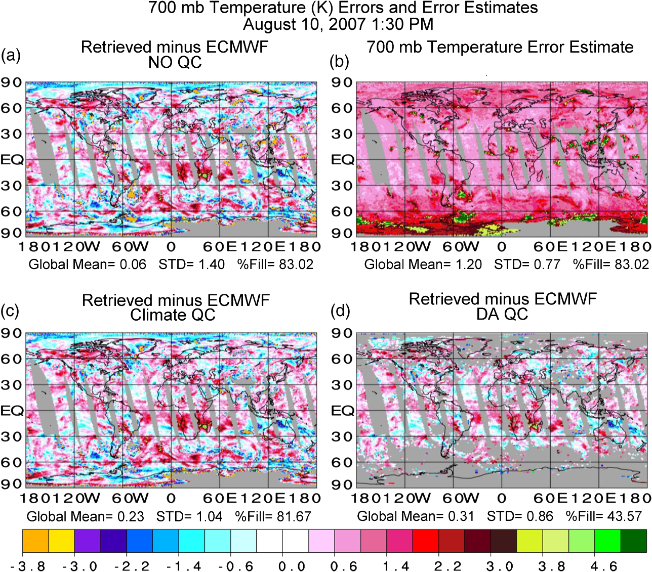 Figures 16(c) and 16(d) show the spatial coverages of QC’d values of with climate QC (,1) and DA QC (), respectively. Of all grid boxes, 81.67% contain values of passing climate QC, which corresponds to 98% of the grid boxes containing AIRS observations. The standard deviation of the errors in the level-3 700 mb temperatures, as compared to ECMWF, has dropped from 1.40 K without QC to 1.04 K using climate QC. Of all grid boxes, 43.57% contain values of 700 mb temperature passing DA QC, which corresponds to 52% of all grid boxes observed by AIRS. The standard deviation of the errors in these grid boxes has dropped to 0.86 K. Analogous figures for version-6 AO, not shown, are very similar to those for version-6. The yield and error statistics shown in Fig. 16 are similar to those shown in Fig. 6 for nine days of level-2 retrievals, in which the 700 mb pressure is indicated by the lower of the two thin horizontal black lines. We have performed principal component analyses of the contributions of the terms involving all predictors in each spatial domain to the 1:30 p.m. 700 mb temperature error estimates shown in Fig. 16(b). These indicate that over nonfrozen ocean, the three largest contributions to the error estimates during the day at 700 mb, in decreasing order of importance, are (1) , indicative of how well the temperature profile retrieval step converged; (2) , the channel noise amplification factor obtained in the final cloud clearing step; and (3) , indicative of how well the water vapor retrieval step converged. The three largest contributions to 700 mb temperature error estimates over land during the day are (1) ; (2) , indicative of how well the cloud clearing step done to generate the values of used in the final physical retrieval step converged; and (3) . The three largest contributions to the daytime 700 mb temperature error estimates over frozen ocean and snow-covered land are (1) ; (2) ; and (3) , indicative of how well the brightness temperature for AMSU channel 6, computed from the final retrieved state, agrees with the observed AMSU channel 6 brightness temperature. This finding is shown for demonstrative purposes only. The relative contributions of predictors to error estimates of different geophysical parameters are not the same as those for 700 mb temperature. Error estimates are generated in a manner different from that used for , , and , as described in the next section. The error estimates are written out as part of the version-6 data set, but are not used in the generation of QC flags for . In version-6, the QC flags for for case are set to be identical to those of for that case. A.2.Generation of Empirical Error Estimates δError estimates for , , are generated empirically in version-6 in a manner analogous to what was done in version-5, according to Eq. (8). where are a subset of seven of the error estimates for derived for that case. The seven error estimate predictors used in Eq. (8) are (1) ; (2) ; (3) ; (4) ; (5) ; (6) ; and (7) . The coefficients are generated in a fashion analogous to those in Eq. (7) using ECMWF values of as truth and minimizing the RMS fractional errors , where is given by . In version-6, as with , , and , coefficients of six distinct matrices, corresponding to daytime and nighttime cases for each of the three geophysical domains described previously, are derived. We use the simplified form of Eq. (8) to derive rather than the form of Eq. (7), involving more predictors, because we felt that errors in temperature profile and total precipitable water for a given case should be adequate predictors of errors in the water vapor profile. The error estimates , which are written out for a given case, are computed according to .A.3.Error Estimates and Quality Control for Clear Column RadiancesThe clear column radiance for channel , , is a derived quantity obtained as part of the version-6 physical retrieval process. Values of and are generated for all operable AIRS channels in those cases where a successful retrieval is produced ( of all cases). The AIRS/AMSU version-6 retrieval algorithm performs one retrieval per AMSU field of regard (FOR), which contains nine AIRS fields of view (FOVs). Each AIRS FOV (, 9) within the AMSU FOR has an observed radiance for each channel , . The observations are potentially affected by clouds in FOV . represents the best estimate of what the observed AIRS channel radiance, averaged over the nine FOVs in the AMSU FOR, would have been if all FOVs were completely cloud free. In version-5 and version-6, is obtained according to where is the average value of over the nine FOVs and (, 9) is a derived vector for each FOR obtained as part of the retrieval process.If all values of used in Eq. (9) were perfect, then the error in would be where is the spatially random noise of channel and is the channel noise amplification factor, resulting from taking the linear combination of observations in the nine FOVs, shown in Eq. (9), to obtain . It can be shown that the appropriate value of is given byEquation (9) shows that if all are zero. This situation occurs whenever observed radiances for channel are thought by the retrieval algorithm to be unaffected by possible cloud cover in the FOR, and the clear column radiance is obtained by averaging the observed channel radiances in all nine FOVs. Equation (11) reduces to when all are zero. In general, this is not the case and is usually , depending on the extent of cloud clearing (extrapolation) performed in the FOR. is, in principle, channel independent because it arises only from the linear combination of radiances used to construct . Nevertheless, some channels are only sensitive to the atmosphere at pressures sufficiently lower than the cloud top pressure (altitudes higher than the cloud top height), and these case-dependent channels do not see the clouds. The retrieval algorithm determines which channels do not see clouds, and for these channels, the retrieval algorithm sets and also sets . Equation (11) is used to generate for all other channels. In general, the largest source of noise in results from errors in the vector . In version-6, as was done in version-5, is expressed as the sum of the errors arising from both sources and , where represents the portion of the predicted clear column radiance error arising from cloud clearing errors. is generated in a manner described in the next section. A.3.1.Clear column brightness temperatures and their error estimatesClear column radiances and their associated error estimates are written out in radiance units (). It is more convenient, however, to think in terms of clear column brightness temperatures , and their error estimates , both given in Kelvin. The clear column brightness temperature is defined as the equivalent blackbody temperature of , which is the temperature such that , where is the Planck blackbody function. As with regard to , we express as the sum of two components and , according to The seven predictors used in Eq. (12) to generate the empirical error estimate term are identical to those used in Eq. (8) to generate . For those channels in which is set equal to , we do not use the second term in Eq. (13) and we write Given , is computed according to is written out as part of the output file but is not used directly for QC purposes. QC is done in terms of in a manner described in the next section.As in the generation of other empirical error estimates, version-6 and version-6 AO use six different matrices in Eq. (12), one for each of six different spatial and temporal domains. The coefficients of the six different matrices are determined analogously to those of the other matrices described previously, such that the coefficients minimize the RMS differences of , where and is computed using Eq. (12). Cases for which Eq. (13) is used to generate are not included in the generation of . The true clear column brightness temperature is taken to be the value of that is computed using the AIRS radiative transfer algorithm in conjunction with the truth state . We used ECMWF 3-h forecast values for , , , and . The profile used in the calculations had a spatially homogeneous vertically constant mixing ratio, which was set to be 371.79 ppm on January 1, 2002, and increased linearly in time at a rate of . The truth values used for , , and were based on spatially varying monthly mean climatologies. The AIRS science team model was used as truth for surface emissivity over nonfrozen ocean. Reasonable globally homogeneous surface emissivity values were used as truth over land. Values of , and, therefore, of , are most accurate for channels in the 15 and 4.3 μm bands, especially those channels that are less sensitive to surface emission. For this reason, the best error estimate coefficients, and subsequent error estimates, are generated in the 15 and 4.3 μm bands for those channels that are not sensitive to surface emission. Error estimate coefficients generated for channels that are very sensitive to water vapor or ozone absorption are less accurate because of limitations in the truth values used for water vapor and ozone profiles. Error estimate coefficients for those channels that are very sensitive to surface emission are also less reliable, but are better over ocean than over land. Finally, clear column radiances at frequencies are affected by incoming solar radiation reflected back in the direction of the satellite by the surface. The relevant surface bidirectional reflectance term is not modeled well in the computation of . For this reason, daytime values of for frequencies between 2180 and , and between 2380 and , are of lower accuracy because radiances in these channels are sensitive to solar radiation reflected by the Earth’s surface in the direction of the satellite. Therefore, for those channels, we substituted the values of determined during nighttime conditions into the daytime matrices , instead of using the values that were computed during daytime conditions. A.3.2.QC flags forDifferent channels are sensitive, by varying amounts, to clouds at different pressures. Therefore, is both channel and case dependent. Even if significant cloud clearing errors exist for some channels in a given case, channels that have little or no sensitivity to the clouds in that case would have very accurate values of . It is for this reason that we assign each channel its own case-dependent QC flags indicating whether the cloud cleared radiance is of sufficient accuracy for use for different purposes. We used the predicted clear column brightness temperature error to assign the QC flags for on a case-by-case basis. In version-6 and version-6 AO, is assigned the flag if is , and is assigned the QC flag if is between 1.0 and 2.5 K. Otherwise, the QC flag is set equal to 2. The flag is intended to mark those channels that are thought to be accurate enough for DA purposes, with the goal that the error in should not be much larger than the channel noise . The flag is designed to provide better spatial coverage for a given channel for use in process studies, but still eliminate poor values of . Figure 15 shows acceptance yields and RMS errors of QC’d values of from 650 to , in which the QC procedures used are as defined in this section. AcknowledgmentsThis work was supported by NASA under the AIRS Science Team proposal “Improved AIRS/AMSU soundings, clear column radiances, error estimates and quality control for use in weather and climate studies (09-TERRAQUA09-0099). ReferencesJ. SusskindC. D. BarnetJ. M. Blaisdell,
“Retrieval of atmospheric and surface parameters from AIRS/AMSU/HSB data in the presence of clouds,”
IEEE Trans. Geoscience and Remote Sens., 41 390
–409
(2003). http://dx.doi.org/10.1109/TGRS.2002.808236 IGRSD2 0196-2892 Google Scholar
J. Susskindet al.,
“Accuracy of geophysical parameters derived from atmospheric infrared sounder/advanced microwave sounding unit as a function of fractional cloud cover,”
J. Geophys. Res., 111 D09S17
(2006). http://dx.doi.org/10.1029/2005JD006272 JGREA2 0148-0227 Google Scholar
J. Susskindet al.,
“Improved temperature sounding and quality control methodology using AIRS/AMSU data: the AIRS science team version-5 retrieval algorithm,”
IEEE Trans. Geosci. Remote Sens., 49 883
–907
(2011). http://dx.doi.org/10.1109/TGRS.2010.2070508 IGRSD2 0196-2892 Google Scholar
S. DeSouza-Machadoet al.,
“Fast forward radiative transfer model of 4.3 um non-local thermodynamic equilibrium effects for the aqua/AIRS infrared temperature sounder,”
Geophys. Rev. Lett., 34 L01802
(2007). http://dx.doi.org/10.1029/2006GL026684 GPRLAJ 0094-8276 Google Scholar
M. T. Chahine,
“Remote sensing of cloudy atmospheres. I. The single cloud layer,”
J. Atmos. Sci., 31 233
–243
(1974). http://dx.doi.org/10.1175/1520-0469(1974)031<0233:RSOCAI>2.0.CO;2 JAHSAK 0022-4928 Google Scholar
M. T. Chahine,
“Remote sensing of cloudy atmospheres. II. Multiple cloud formations,”
J. Atmos. Sci., 34 744
–757
(1977). http://dx.doi.org/10.1175/1520-0469(1977)034<0744:RSOCAI>2.0.CO;2 JAHSAK 0022-4928 Google Scholar
Z. TaoW. J. BlackwellD. H. Staelin,
“Error variance estimation for individual geophysical parameter retrievals,”
IEEE Trans. Geosci. Remote Sens., 51 1718
–1727
(2013). http://dx.doi.org/10.1109/TGRS.2012.2207728 IGRSD2 0196-2892 Google Scholar
W. J. Blackwell,
“Neural network Jacobian analysis for high-resolution profiling of the atmosphere,”
EURASIP J. Adv. Signal Process.,
(2012). http://dx.doi.org/10.1186/1687-6180-2012-71 Google Scholar
E. T. Olsenet al., AIRS/AMSU/HSB Version 6 Retrieval Flow, Jet Propulsion Laboratory, Pasadena, CA
(2013). Google Scholar
X. WuW. L. Smith,
“Emissivity of rough sea surface for 8–13 um: modeling and verification,”
Appl. Opt., 36 2609
–2619
(1997). http://dx.doi.org/10.1364/AO.36.002609 APOPAI 0003-6935 Google Scholar
W. W. Seemanet al.,
“Development of a global infrared land surface emissivity database for application to clear sky sounding retrievals from multi-spectral satellite radiance measurements,”
J. Appl. Meteorol. Climatol., 47 108
–123
(2008). http://dx.doi.org/10.1175/2007JAMC1590.1 1558-8424 Google Scholar
J. SusskindO. Reale,
“Improving forecast skill by assimilation of AIRS temperature soundings,”
in 2010 IEEE Intl. Geoscience and Remote Sensing Symp.,
3534
–3537
(2010). Google Scholar
B. H. Kahnet al.,
“The atmospheric infrared sounder version 6 cloud products,”
Atmos. Chem. Phys., 14 399
–426
(2014). http://dx.doi.org/10.5194/acp-14-399-2014 ACPTCE 1680-7316 Google Scholar
J. Susskindet al.,
“Interannual variability of outgoing longwave radiation as observed by AIRS and CERES,”
J. Geophys. Res., 117 D23107
(2012). http://dx.doi.org/10.1029/2012JD017997 JGREA2 0148-0227 Google Scholar
M. J. Iaconoet al.,
“Radiative forcing by long-lived greenhouse gases: calculations with the AER radiative transfer models,”
J. Geophys. Res., 113 D13103
(2008). http://dx.doi.org/10.1029/2008JD009944 JGREA2 0148-0227 Google Scholar
A. V. MehtaJ. Susskind,
“Outgoing longwave radiation from the TOVS pathfinder path A data set,”
J. Geophys. Res., 104 12193
–12212
(1999). http://dx.doi.org/10.1029/1999JD900059 JGREA2 0148-0227 Google Scholar
E. T. Olsenet al., AIRS/AMSU/HSB Version 6 Data Release User Guide, Jet Propulsion Laboratory, Pasadena, CA
(2013). Google Scholar
E. M. ManningS. Z. Friedman, AIRS Version 6.0 Released Files Description, Jet Propulsion Laboratory, Pasadena, CA
(2013). Google Scholar
BiographyJoel Susskind is a senior scientist in the Laboratory for Atmospheres at the NASA Goddard Space Flight Center, where he has worked since 1977 doing research in infrared and microwave remote sensing. He is a member of the AIRS Science Team and is conducting research aimed at improving products derived from AIRS observations and using AIRS sounding products to further improve numerical weather prediction as well as to study climate processes and trends. John M. Blaisdell received a BA in mathematics and BS in physics from the University of Rochester, and MS and PhD degrees in physics from the University of Illinois. He joined Science Applications International Corporation/General Sciences Corporation in 1983, working on space and atmospheric applications, including the Hubble Space Telescope and Tropical Rainfall Measuring Mission. Since 1993, he has supported the Sounder Research Team at NASA Goddard Space Flight Center, implementing atmospheric sounding algorithms. Lena Iredell received a BS in meteorology from SUNY Oswego and a MS in forest micrometeorology from West Virginia University. Her area of expertise includes the development of quality control methodologies, development of level-3 gridding algorithms, statistical and graphical analysis, and validation of retrieved surface and atmospheric products from the AIRS/AMSU and TOVS instruments. She started at NASA Goddard in 1981 and supports the atmospheric-sounding research activities of the Sounder Research Team. |
|||||||||||||||||||||||||||||||||||||||||||||||||||||||||||||||||||||||||||||||||||||||||||||||


