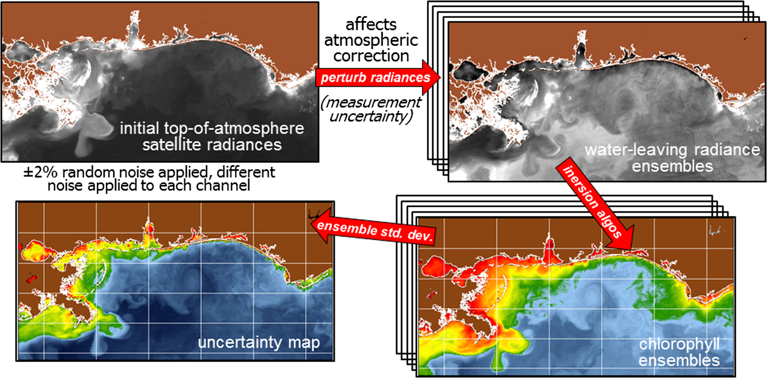2.1.

Satellite Imagery/Processing

The Naval Research Laboratory (NRL) at the Stennis Space Center (SSC) in Mississippi has developed an automated processing system (APS) that ingests and processes AVHRR, SeaWiFS, MODIS, MERIS, OCM, HICO, and VIIRS satellite imagery.¹⁷ APS is a powerful, extendable, and image-processing tool. It is a complete end-to-end system that includes sensor calibration, atmospheric correction (with NIR correction for coastal waters), and bio-optical inversion. APS incorporates the latest NASA MODIS code and enables us to produce the NASA standard MODIS products, as well as Navy-specific products using NRL algorithms. We can quickly reprocess many data files (hundreds of scenes/day), and we maintain compatibility with NASA/Goddard algorithms and processing code in the SeaWiFS Data Analysis System (SeaDAS); APS is updated as SeaDAS is updated.

All imagery was processed with consistent atmospheric correction and bio-optical algorithms using the NRL APS Version 4.6, which is consistent with SeaDAS Version 6.3 (both SeaDAS and APS have been modified and updated). The OC3M algorithm was used to estimate chlorophyll concentration;⁴ it requires radiances at 443, 488, and 547 nm. Thus, adding noise to the other MODIS visible wavelengths will not directly impact the chlorophyll estimates (the other visible wavelengths are used in other bio-optical algorithms, but those are not presented here). However, an iterative, NIR atmospheric correction tuned for coastal waters was applied,¹⁸ as was a correction for absorbing aerosols.¹⁹ Perturbing the 667-nm radiances has an effect on the NIR atmospheric correction, and the absorbing aerosol correction can potentially affect radiance values at all the visible wavelengths [the absorbing aerosol algorithm increases normalized water-leaving radiances (nLw) (with greater increases at blue wavelengths) by reducing the aerosol radiance subtracted during the atmospheric correction]. Thus, application of these algorithms will indirectly affect the chlorophyll estimates.

With the NRL APS, the architecture is in place for the image ensemble analysis. From an initial MODIS image, we simply create an ensemble of new images by applying the $\pm 2\%$ random noise to the TOA radiance values. Each ensemble image is then reprocessed through APS to yield an ensemble of derived products, such as ${{}_{\mathrm{n}}L}_{\mathrm{w}}$ and chlorophyll (that we examine here) among others.

2.2.

Hydrodynamic Model

To advect the surface MODIS satellite chlorophyll field and produce 24-, 48-, and 72-h forecast simulations, we used currents derived from the Relocatable Navy Coastal Ocean Model (RELO-NCOM). RELO-NCOM is based on a standardized development and an efficient configuration management to facilitate transitions of new tools and real-time configurations of regional high-resolution (order 1 km) ocean predictions. The physics and numerical procedures of NCOM are based on the Princeton Ocean Model and a Sigma/Z-level Model (SZM). It solves a three-dimensional (3-D), primitive equation, baroclinic, hydrostatic and free surface system using a Cartesian horizontal grid, a combination of $\sigma /z$ level (i.e., bottom-following/constant depth) vertical grid, and implicit treatment of the free surface.²⁰ It uses the Mellor–Yamada level 2.5 turbulence closure scheme, and the Smagorinsky formulation for horizontal mixing.²¹ For mesoscale real-time applications, boundary conditions are taken from an operational run of the global NCOM (GNCOM). The domain of this particular experiment covered the entire Gulf of Mexico (18°N 98°W, 40°N 79°W), from April 1, 2011, to October 30, 2011. The atmospheric forcing was taken from the regional 15-km coupled ocean/atmosphere mesoscale prediction system run by the Fleet Numerical Meteorological and Oceanographic Center. Tides were introduced at the boundaries and through local tidal potentials. The horizontal grid spacing was set at 3 km and used 50 $\sigma /z$ levels in the vertical. The model assimilates local in situ observations along with satellite altimetry and sea-surface temperature data using a combination of model analysis and data; all available observations from global and local databases were assimilated over the full period.

For the chlorophyll forecasts, a “pseudo 3-dimensional” Eulerian advection scheme was used (without molecular or turbulent diffusion terms). With this approach, there are essentially two vertical layers, a 1-m-thick surface layer and a conceptual deep layer to preserve continuity (i.e., there is vertical flux between the two layers, but they move together horizontally). These simulations only include current advection and an assumed uniform vertical chlorophyll distribution based on the surface values. Future enhancements will include addition of diffusion terms, full 3-D vertical layering, and the capability to include more realistic vertical chlorophyll profiles. The forecast simulations do not include any assimilation of in situ chlorophyll data or additional satellite imagery, so currently the values are unconstrained. Also, with this approach, there is an implicit assumption that the bio-optical property (chlorophyll) is conservative. Although this is not strictly true, of course, it may be approximately valid over the short time scales (1–3 days) that we are examining, particularly in coastal areas where transport processes might be expected to dominate biological processes. Therefore, we consider the optical properties to be “pseudo-conservative” tracers for our purposes. This allows us to ignore growth and grazing terms for this case and treats the distributional changes as though they are entirely due to dynamical processes.²²

3.1.

Generating Ensembles

Figure 1 illustrates the process we used to generate ensembles for an ocean color satellite image. As mentioned above, we generated a suite of 100 individual chlorophyll ensemble members from a single image by randomly applying $\pm 2\%$ noise to the TOA radiances in the visible and NIR bands. Different random noise was applied to each band, but there was no variation from pixel to pixel (i.e., it was constant across the scene). By perturbing the radiances, we are simulating measurement uncertainty or sensor degradation, which affects the atmospheric correction process and subsequently the downstream water-leaving radiance estimates (and eventually the derived bio-optical products, following application of the bio-optical inversion algorithms). Thus, from the single original image, we create a set of 100 separate chlorophyll estimates, each representing some deviation from the unperturbed chlorophyll estimate. We then calculate the standard deviation at each pixel using this image set, and we use this estimate of variability as a proxy for uncertainty. The assumption here is that the ensemble set is realistic, that we are applying a reasonable amount of noise to the radiances, and that the noise encompasses natural variability. We need to test this assumption, to ensure that the ensemble variability will represent accurate estimates of product uncertainties.

As an example test case to demonstrate the methodology, we selected a clear MODIS image covering the northern Gulf of Mexico (October 14, 2011). Figure 2(a) shows the chlorophyll image from the unperturbed, original image following standard processing (consistent with NASA algorithms). The mean chlorophyll image from the 100-member ensemble suite is shown in Fig. 2(b), and the associated uncertainty image (the ensemble standard deviation) is shown in Fig. 2(c). Note that the ensemble mean image looks very similar to the unperturbed chlorophyll image, as we would expect if our ensemble suite is realistic.

Fig. 2

MODIS October 14, 2011, Mississippi Bight region (a) chlorophyll, original image, standard processing, (b) mean ensemble chlorophyll, and (c) ensemble chlorophyll standard deviation (proxy for uncertainty). For the ensemble suite, 100 ensemble members were generated, with $\pm 2\%$ random noise applied to the $L_{\mathrm{t}}$ values for the visible and NIR wavelengths.

3.2.

Assessing Ensemble Representativeness

An initial step with the use of ensembles is to assess whether the ensemble suite adequately represents reality. In other words, is the ensemble variability representative of natural variability? For this assessment, since we applied noise to the image TOA radiances ($L_{\mathrm{t}}$), we compared the ensemble $L_{\mathrm{t}}$ radiances (mean, minimum, and maximum values) to the $L_{\mathrm{t}}$ radiances from the original image (nearly identical; not shown), and to $L_{\mathrm{t}}$ radiances derived from selected clear MODIS scenes covering the same area over a 2-year period from 2006 to 2007 (Fig. 3). We refer to the 2-year values as climatological values. The values in Fig. 3 are spatial averages across the Mississippi Bight region (i.e., the entire scene in Fig. 2), as well as temporal averages over the 2-year period for the climatology. For the most part, the ensemble mean and the minimum/maximum values fall within the envelope of variability described by the climatology. Hence, the ensemble suite is not generating “unusual” variability outside the realm of observed natural variability, and our assessment is that the ensemble suite is realistic. However, the $L_{\mathrm{t}}$ radiances for this image (original as well as ensemble mean values) are lower than the climatological means at all wavelengths (solid red versus solid blue lines, Fig. 3).

Fig. 3

$L_{\mathrm{t}}$ radiance (mean, minimum/maximum values) versus wavelength, averaged spatially across the entire Mississippi Bight region (shown in Fig. 2). Climatological radiances (from 2-year MODIS climatology covering 2006–2007) and ensemble radiances (generated from October 14, 2011 image).

We also examined the effect of the $L_{\mathrm{t}}$ noise on the derived ${{}_{\mathrm{n}}L}_{\mathrm{w}}$ values, to verify that the radiance values following atmospheric correction were also realistic. Again, we compared the ensemble values to the original values [Fig. 4(a)] and the climatological values [Fig. 4(b)]. These are mean values averaged across the entire image, as in Fig. 3. The mean ensemble ${{}_{\mathrm{n}}L}_{\mathrm{w}}$ values at the short wavelengths are slightly higher than the original values [Fig. 4(a)]. Both the ensemble and original ${{}_{\mathrm{n}}L}_{\mathrm{w}}$ values are significantly lower than the climatological values at 412 nm, but the mean and standard deviation values are generally similar at the other wavelengths [Fig. 4(b)].

Fig. 4

${{}_{\mathrm{n}}L}_{\mathrm{w}}$ radiance ($\text{mean}\pm \text{standard deviation}$) versus wavelength, averaged spatially across the entire Mississippi Bight region (shown in Fig. 2) a) original October 14, 2011 radiances and ensemble radiances and b) climatological radiances and ensemble radiances.

To more closely examine the ${{}_{\mathrm{n}}L}_{\mathrm{w}}$ spectral variability of the ensemble suite, and to further assess the validity of the ensembles, we compared the individual ensemble spectra to the spectrum of the original, unperturbed MODIS image, at two locations (instead of looking at spatial and temporal averages, as in Figs. 3 and 4). The first location is a coastal aerosol robotic network (AERONET) site in the northern Gulf of Mexico (28.867°N, 90.483°W; http://aeronet.gsfc.nasa.gov/new_web/photo_db/WaveCIS_Site_CSI_6.html). Coincident in situ ${{}_{\mathrm{n}}L}_{\mathrm{w}}$ measurements collected over 3 years (2010–2012) are available at this site, for comparison to the image spectra [Fig. 5(a)]. The second location is a randomly selected, clear water, open-ocean site [28.75°N, 86.5°W; Fig 5(a)] to provide a contrast to the more turbid coastal site; there were no coincident in situ measurements at this location. The ensemble and original spectra were extracted and averaged over $3\times 3\text{pixel}$ boxes centered at the AERONET and open-ocean locations.

Fig. 5

${{}_{\mathrm{n}}L}_{\mathrm{w}}$ radiance versus wavelength. Comparison of 100 individual ensemble members (black lines) with ensemble $\text{mean}\pm \text{standard deviation}$ (red lines) and original, unmodified spectrum (blue line) from the same location, for October 14, 2011 MODIS image a) coastal AERONET (WaveCIS) location. 3-year $\text{mean}\pm \text{standard deviation}$ of in situ data (green lines) is also overlaid and b) open-ocean location (NOTE: no in situ data for comparison at this location).

At the AERONET location, the ensemble mean and standard deviation [Fig. 5(a), solid and dashed red lines, respectively] fall within the observed envelope of measured variability from the in situ data set (3-year mean and standard deviation, solid and dashed green lines, respectively), for most wavelengths. Note that the purpose of this comparison is not to validate the satellite data against the AERONET data, but simply to demonstrate that the generated ensembles are realistic and not outside the longer-term envelope of variability for the region. However, the mean ensemble ${{}_{\mathrm{n}}L}_{\mathrm{w}}$ spectral shape differs from the in situ measured spectral shape; relative to the AERONET mean spectrum, the ensemble mean spectrum has higher ${{}_{\mathrm{n}}L}_{\mathrm{w}}$ values at 443 nm and lower values at 531 nm (the individual ensemble spectra match this pattern as well). The ${{}_{\mathrm{n}}L}_{\mathrm{w}}$ spectral shape from the original, unperturbed image (blue line), also follows this pattern; however, indicating that the differences in the ensemble versus in situ spectral shapes are not due to improper ensemble generation, but due to differences between the original versus in situ spectral shapes.

As at the AERONET site, the ensemble mean spectrum at the open-ocean site [Fig. 5(b), solid red line] closely matches the original spectrum (blue line), although the ensemble values are slightly higher than the original spectrum at 412 and 443 nm. Note that at both sites, the spectral shapes of the individual ensemble members can differ significantly from the mean spectrum. In some cases, the individual spectra are not even realistic, particularly in the 443- to 547-nm wavelength range at the AERONET location, and in the 412- to 488-nm range at the open-ocean location. These spectral shape differences will undoubtedly lead to widely varying and probably unrealistic chlorophyll values derived from the individual spectra (although the mean spectrum is fine) and point to the need for spectral constraints when generating the noise ensembles; this is discussed further below and it is a topic of our current research.

Since the ultimate goal is to derive water bio-optical properties from the ocean color imagery, we further compared the chlorophyll frequency distribution from the original, unperturbed image to the ensemble frequency distribution [log chlorophyll; Fig. 6(a)]. As a result of the slightly higher ${{}_{\mathrm{n}}L}_{\mathrm{w}}$ radiances for the ensemble mean at blue wavelengths (412 and 443 nm) compared to the original values [Fig. 4(a)], the ensemble chlorophyll values are slightly lower than the original chlorophyll values, i.e., the chlorophyll distribution is skewed to slightly lower values across the scene [Fig. 6(a)]. This is also apparent in the frequency distribution of the percent differences between the original chlorophyll values and the ensemble chlorophyll values [Fig 6(b)]. The ensemble mean chlorophyll value is about 5% lower than the original value (ranges from about 15% lower to about 5% higher than the original chlorophyll).

Fig. 6

Chlorophyll frequency distributions, ensemble mean versus original (a) log chlorophyll values and (b) percent difference between ensemble mean and original chlorophyll values.

These results indicate that although our mean $L_{\mathrm{t}}$ and ${{}_{\mathrm{n}}L}_{\mathrm{w}}$ ensemble variability falls within the range of variability observed in the climatology and in situ data sets, the “unconstrained” spectral noise on the $L_{\mathrm{t}}$ values might be creating some unrealistic individual ensemble members. By “unconstrained,” we mean that the noise applied to one wavelength is independent of the noise applied to another wavelength, which could potentially lead to the undesirable effect of creating $L_{\mathrm{t}}$ spectral shapes (and subsequently ${{}_{\mathrm{n}}L}_{\mathrm{w}}$ spectral shapes) that are not realistically observed in nature (e.g., see some of the individual ensemble spectra in Fig. 5). This effect would be particularly troublesome at blue and green wavelengths, since the spectral shape in this portion of the spectrum determines the blue–green ratio, which is used in the OC3M chlorophyll algorithm. Furthermore, a 2% increase in $L_{\mathrm{t}}$ at 443 nm and a 2% decrease at 547 nm has a more significant impact on the chlorophyll retrieval than a 2% increase at both wavelengths. Thus, these altered spectral shapes could significantly change the derived chlorophyll value. We are currently developing a method to apply spectral constraints during the generation of the $L_{\mathrm{t}}$ ensembles that should eliminate the erroneous individual spectral shapes and yield an ensemble chlorophyll frequency distribution that is more consistent with the original distribution.

In Fig. 6, we compared the ensemble mean chlorophyll to the original chlorophyll (from the unperturbed image) and observed that, on average, the ensemble chlorophyll was slightly less than the original chlorophyll. We have also compared the ensemble chlorophyll range to the climatological range observed in the 2-year MODIS climatology. Figure 7 shows the spatial distributions of the differences between the ensemble minimum chlorophyll value at each pixel and the climatological minimum chlorophyll value [Fig. 7(a)], and the difference between the climatological maximum chlorophyll value and the ensemble maximum chlorophyll value [Fig. 7(b)]. Pixels in yellow indicate areas where the ensemble range (minimum or maximum) falls outside of the climatological range. The minimum ensemble chlorophyll values fall slightly below the minimum climatological chlorophyll values at many of the offshore pixels [Fig. 7(a)], suggesting again that perhaps the ensembles require adjustment (through application of spectral constraints to the $L_{\mathrm{t}}$ noise values applied).

Fig. 7

Comparison of ensemble chlorophyll range to climatological range: (a) ensemble minimum chlorophyll−climatological minimum chlorophyll. Yellow pixels indicate the minimum ensemble chlorophyll value is lower than the climatological minimum value and (b) climatological maximum chlorophyll−ensemble maximum chlorophyll. Yellow pixels indicate the maximum ensemble chlorophyll value is higher than the climatological maximum value.

3.3.

Partitioning Chlorophyll Differences and Uncertainties

We examined the spatial distributions of the differences between the mean ensemble and original chlorophyll values; Fig. 8 shows the percent differences between the two. We first apply noise to the $L_{\mathrm{t}}$ values in both the visible and NIR channels [Fig. 8(a)]. This demonstrates the noise impact on the complete processing. Then, by only applying noise to the $L_{\mathrm{t}}$ values in the two NIR bands (748 and 869 nm), we can assess the effects of the noise only due to the atmospheric correction process [i.e., differences due to different aerosol selection models, Fig. 8(b)]. Similarly, by only applying noise to the visible channels (412, 443, 488, 531, 547, 667, and 678 nm), we can assess the effects of the noise on the bio-optical inversion algorithms [Fig. 8(c)]. Figure 8(a) indicates that the mean ensemble chlorophyll values are generally lower than the original chlorophyll values across most of the image, by about 5–10% (mean difference, averaged across the entire image is $-4.8\%$ when noise is applied to all channels [which is consistent with Fig. 6(b)]. A much lower percent difference is observed when noise is applied to just the NIR channels [$\text{mean difference}=-0.5\%$, Fig. 8(b)]. When noise is applied to just the visible wavelengths [Fig. 8(c)], the mean difference is $-4.3\%$, indicating that a relatively larger proportion of the observed chlorophyll differences is due to the bio-optical inversion algorithms, rather than the atmospheric correction.

Fig. 8

Percent difference between the ensemble mean chlorophyll and the original chlorophyll for the October 14, 2011 MODIS image (a) $L_{\mathrm{t}}$ noise applied to both NIR and visible wavelengths, (b) $L_{\mathrm{t}}$ noise applied to just NIR wavelengths, and (c) $L_{\mathrm{t}}$ noise applied to only the visible wavelengths. Blue pixels indicate that the original chlorophyll values were higher than the ensemble values, yellow pixels, vice versa. White pixels indicate agreement within $\pm 2\%$.

Using the noise partitioning approach described above (for Fig. 8), we can also examine the separate effects of the atmospheric correction and bio-optical inversions on the uncertainty distributions (Fig. 9). Figure 9(a) shows the coefficient of variation (CV) expressed as a percentage (CV, the ratio of the standard deviation to the mean * 100) across the image, when $L_{\mathrm{t}}$ noise is applied to all wavelengths (both visible and NIR). The mean CV across the image is 33.6%. Figure 9(b) shows the result when noise is applied only to the NIR bands (mean $\mathrm{CV}=11.5\%$), and Fig. 9(c) shows the results for noise applied only to the seven visible bands (mean $\mathrm{CV}=30.8\%$). As in Fig. 8, Fig. 9 indicates that most of the uncertainty is associated with the bio-optical inversion algorithms (expressed by adding noise to the visible bands), rather than with the atmospheric correction (expressed by adding noise to the NIR bands).

Fig. 9

Chlorophyll coefficient of variation for noise applied to separate band sets (partitioned uncertainty) for the October 14, 2011 MODIS image (a) $L_{\mathrm{t}}$ noise applied to both NIR and visible wavelengths, (b) $L_{\mathrm{t}}$ noise applied to just NIR wavelengths, and (c) $L_{\mathrm{t}}$ noise applied to only the visible wavelengths.

3.4.

Forecasting Chlorophyll, Partitioning Uncertainties, and Assessing Skill

In addition to generating chlorophyll ensembles to create uncertainty maps for the chlorophyll product, we also generated a short-term (3-day) forecast of the chlorophyll distribution (along with an accompanying uncertainty image for the forecast), by coupling the satellite image with current estimates from a hydrodynamic model. To do this, we examined a clear, 3-day period (covering the Mississippi Bight region in the northern Gulf of Mexico) from October 14–17, 2011. This hydrodynamic approach treats the chlorophyll as a passive tracer and only accounts for dynamical processes (winds, currents, and tides) and does not include biogeochemical mechanistic processes (growth and grazing); it allows us to examine the effect of just current variability on the bio-optical forecasts.

We created two sets of ensembles, one set for the ocean hydrodynamic model currents and one set for the initial chlorophyll image to be advected using the currents; by examining them separately or in combination, we can assess the uncertainty in the 3-day forecast due to the uncertainty in the currents (top panel in Fig. 10), or due to the combined uncertainty in the chlorophyll estimate and the currents (bottom panel in Fig. 10). An ensemble of 20 chlorophyll images was generated for the initial October 14 MODIS scene by applying random noise ($\pm 2\%$) to the $L_{\mathrm{t}}$ radiances for all the visible (7) and NIR (2) channels. An ensemble of 32 ocean model members was generated by varying initial and boundary conditions, and atmospheric forcing. Thus, a total of $640(32\times 20)$ chlorophyll forecasts were generated by advecting each of the 20 chlorophyll ensemble members from October 14 for 3 days with each of the 32 ocean current ensembles.

Fig. 10

Schematic illustrating advective bio-optical forecasting approach using only ocean current ensembles (top panel) and using both chlorophyll and ocean current ensemble sets (bottom panel).

In Fig. 11(a), the unperturbed chlorophyll image for October 17 (end of the forecast period) is shown, for comparison to the forecast chlorophyll images. The mean ensemble chlorophyll forecast resulting from the 3-day simulation when only the hydrodynamic uncertainty was included (mean of 32 ensemble members) is shown in Fig. 11(b) for October 17. In this case, we are essentially assuming that the initial chlorophyll image is error-free. The mean ensemble chlorophyll forecast resulting from inclusion of both the hydrodynamic and chlorophyll uncertainties (mean of 640 ensemble members) is shown in Fig. 11(c). Compare Figs. 2(a) to 11(a) to see the observed change in the chlorophyll field over the 3-day period (unperturbed MODIS images for October 14 and 17, respectively). Both of the mean forecast images [Figs. 11(b) and 11(c)] are quite similar, and neither captured the eddy-like feature that likely sheds from the Mississippi River plume and advected toward the east [high-chlorophyll feature near 29°N, 88°W in Fig. 11(a)].

Fig. 11

(a) MODIS image for October 17, 2011 (gray pixels are clouds), (b) forecast ensemble mean chlorophyll for October 17, 2011 (3-day simulation), only hydrodynamic uncertainty included, and (c) forecast ensemble mean chlorophyll for October 17, 2011 (3-day simulation), both hydrodynamic and chlorophyll uncertainties included.

The standard deviation image corresponding to Fig. 11(b), for the simulation including only the hydrodynamic uncertainty, is shown in Fig. 12(a). The highest standard deviation values (i.e., greatest uncertainty in the currents) are along the Mississippi River delta. The standard deviation image corresponding to Fig. 11(c), for the simulation including both the hydrodynamic and chlorophyll uncertainties, is shown in Fig. 12(b). Now, high-standard deviation values are observed along the Louisiana, Mississippi, and Alabama coastlines, in addition to the high values near the delta. Thus, the addition of the chlorophyll uncertainty has increased the forecast uncertainty along the coastlines [i.e., the standard deviation field that would result if image 12(a) was subtracted from image 12(b)]. Figure 12(c) shows the forecast mismatch (i.e., the difference between the forecast and observed chlorophyll distributions, without regard to sign, |Figs. 11(c)–11(a)|), for the forecast that includes both hydrodynamic and chlorophyll uncertainties. If we compare Fig. 12(c) to the corresponding forecast standard deviation [Fig. 12(b)], we see that the patterns match quite well (except for the eddy-like feature mentioned above); the largest ensemble standard deviations correspond to the largest forecast observation mismatches. This indicates that the forecast mismatch is related to both the hydrodynamic and chlorophyll uncertainties and that the chlorophyll is behaving conservatively over most of the image area (i.e., our assumption that the chlorophyll is behaving as a passive tracer over this relatively short time period is valid). Thus, we can account for most of the mismatch by the uncertainties in the currents and in the satellite-derived chlorophyll estimates.

Fig. 12

(a) Forecast ensemble chlorophyll standard deviation for October 17, 2011 (3-day simulation), only hydrodynamic uncertainty included, (b) forecast ensemble chlorophyll standard deviation for October 17, 2011 (3-day simulation), both hydrodynamic and chlorophyll uncertainties included, and (c) forecast mismatch. Forecast ensemble mean chlorophyll for October 17, 2011 (3-day simulation, both hydrodynamic and chlorophyll uncertainties included) minus observed chlorophyll distribution for that day (MODIS image for October 17, 2011), without regard to sign, i.e., |Figs. 11(c)–11(a)|. Black pixels indicate clouds.

By subtracting Fig. 12(b) from Fig. 12(c), we can get an indication of the chlorophyll sources and sinks (Fig. 13). In this figure, the red pixels indicate a chlorophyll “sink,” where observed values were lower than the forecast values, and the blue pixels indicate a chlorophyll “source,” where the observed values were higher than the forecast values. White pixels indicate differences close to 0. These sources and sinks are due to errors in the model currents and/or processes that affect the chlorophyll concentrations that are not accounted for in the model, such as growth and grazing. This image is essentially an assessment of the forecast mismatch after trying to account for the uncertainty. Notice that, except for the eddy feature, the sources and sinks are located along the coast and near the Mississippi River delta. The eddy feature highlighted as a source is most likely due to erroneous current forecasts in that area and probably represents a separation of high-chlorophyll water from the Mississippi River plume, rather than in situ phytoplankton growth.

Fig. 13

Difference image [Figs 12(c)–12(b)], representing source and sinks, where blue pixels represent a chlorophyll source ($\text{observed values}>\text{forecast values}$), and red pixels indicate a chlorophyll sink ($\text{observed values}<\text{forecast values}$). White pixels indicate differences close to 0, and black pixels indicate clouds.

For a more quantitative evaluation of the forecast skill, we can examine spread-skill statistics. Spread-skill scatter plots of the standard deviation of the observed mismatch between the forecast and observed distribution versus the ensemble predicted standard deviation are shown in Fig. 14. Each point in Fig. 14 represents a bin of 1000 pixels. Good spread-skill (a linear distribution following the one-to-one line) indicates that the predicted standard deviation increases with the mismatch standard deviation. For the forecast with only hydrodynamic uncertainty included [Fig. 14(a)], there is good spread-skill at standard deviations less than about 1.6, but deviation from the $1:1$ line are observed at standard deviations above this value. The points above the $1:1$ line indicate sources and sinks not accounted for in the model (i.e., the red and blue pixels in Fig. 13). For the forecast with both hydrodynamic and chlorophyll uncertainties included [Fig. 14(b)], there is improved spread-skill, indicated by the more linear distribution over a larger range (higher coefficient of determination, $R^2$). The distribution of points below the $1:1$ line up to $X$ values of about 2.5 indicates a slight overprediction of uncertainty from the ensembles, whereas the points above the $1:1$ line at higher values indicate an underprediction. In general, the forecast demonstrates good spread-skill with both properties increasing fairly linearly.

Fig. 14

Spread-skill metric plots, observed mismatch standard deviations versus ensemble predicted standard deviations (a) 3-day simulation, only hydrodynamic uncertainty included, and (b) 3-day simulation, both hydrodynamic and chlorophyll uncertainties included.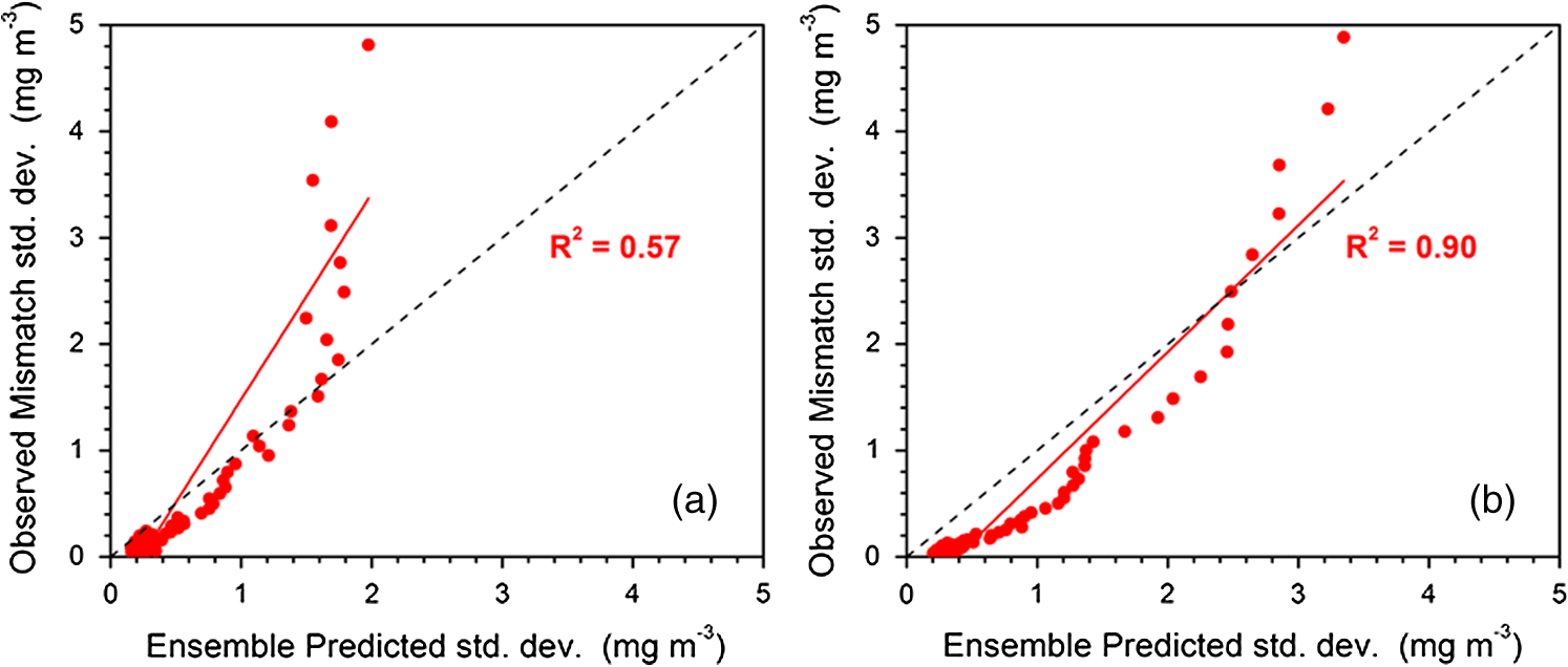

Finally, we examine the ensemble root-mean-square (RMS) difference to assess the spread of the ensemble variability and look for outliers in the ensemble suite (Fig. 15). This matrix represents the RMS difference between an individual ensemble forecast image and the reference image (the unperturbed October 17 image), for each of the 640 ensemble members. The vertical dimension represents the 20 image ensemble members and the horizontal dimension represents the 32 ocean current ensemble members. The horizontal banding at image ensemble members 7 and 18 (higher RMS differences compared to the other image ensemble members) indicates that these two ensemble members have chlorophyll values significantly different from the others. These two are outliers and could be removed (or the image ensemble suite should be adjusted using spectral noise constraints as discussed above) to improve the estimates of the forecast uncertainty.

Fig. 15

Ensemble RMS difference matrix. Vertical dimension represents the 20 image ensemble members, horizontal dimension represents the 32 ocean current ensemble members. Colors represent the RMS difference between the individual ensemble forecast image and the reference image (October 17 unperturbed), for each of the 640 ensembles.