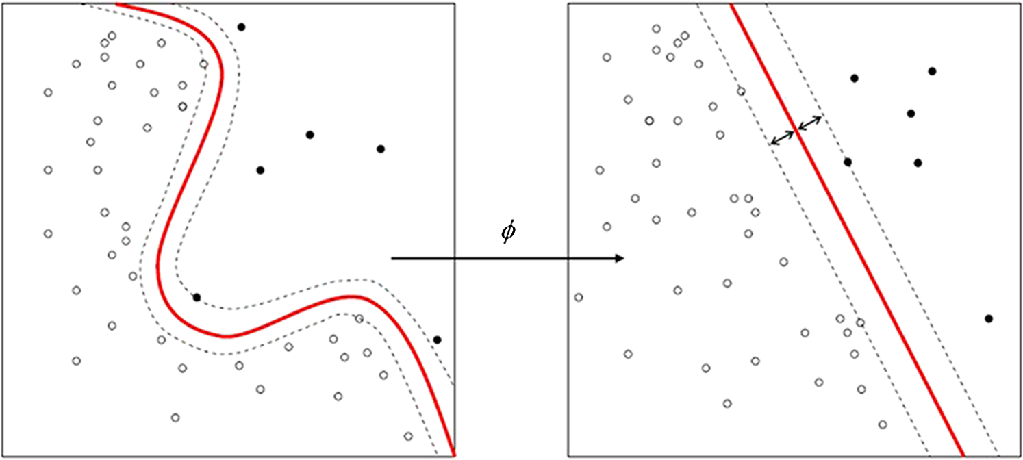
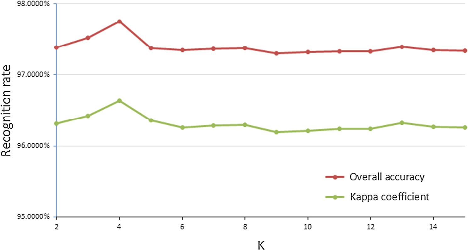
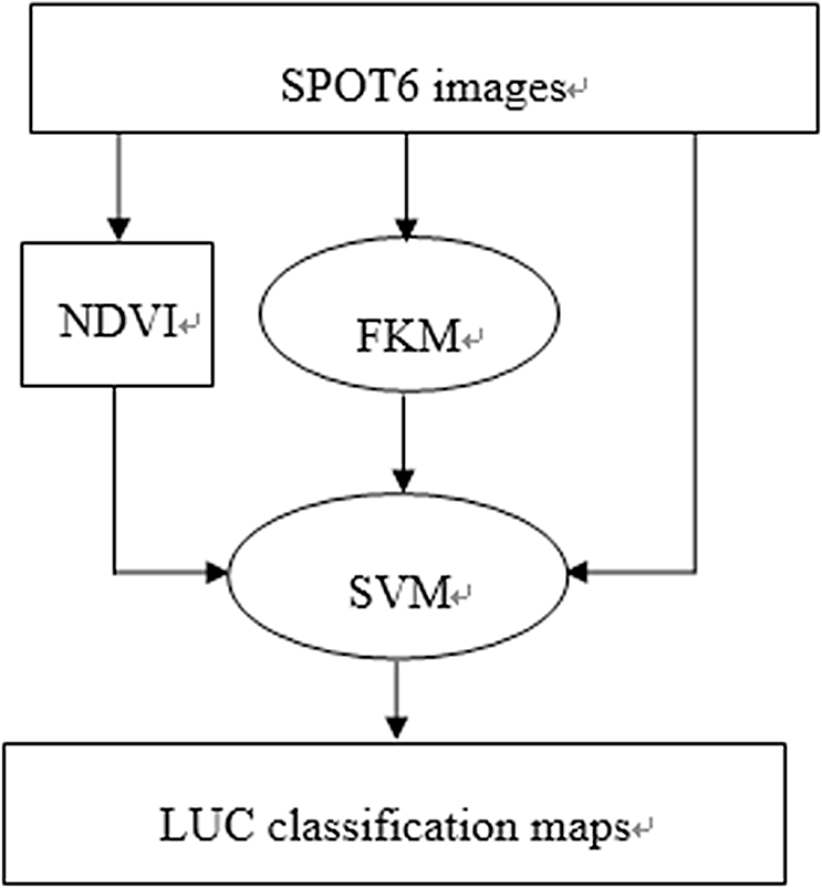
1.

Introduction

Land use/cover (LUC) classification is a key research field in remote sensing, and plays an important role in climate change, biodiversity conservation, and people’s livelihoods. Accurate LUC maps derived from remotely sensed data have become the basis for analyzing many socio-ecological issues.¹ LUC classification is nothing more than a convenient abstraction and may be improved by considering the other lines of evidence, such as surfaces that reflect the range of variability within and between the categories of a classification scheme.²

One basic issue to enhance the LUC classification is to choose an optimal classifier. A series of conventional classification methods have been well developed and long used for remote sensing applications, which are parallelepiped, minimum distance, and maximum likelihood (ML) models.^3–5 Many other advanced classification techniques have also been introduced in the field of remote sensing classification, including artificial neural networks, machine-learning, decision trees, genetic algorithms, and support vector machines (SVM).^6–10

Machine learning algorithms are widely used classification algorithms during the past decades and some assessments of their relative performance compared to other classifiers have been conducted in the Amazon region.^11,12 SVMs (Refs. 13 and 14) have demonstrated their classification accuracies in several remote sensing applications.¹⁵ Specifically, SVMs have been shown to reach high accuracies in LUC mapping and outperform other algorithms.^16–21 The success of such approaches is related to the intrinsic properties of the SVM classifier, which can handle ill-posed problems, and to the curse of dimensionality,²² which provides robust sparse solutions and delineates nonlinear decision boundaries between the classes.

The SVM classifier has a significant advantage for LUC classification. It seeks to separate LUC classes by finding a plane in the multidimensional feature space that maximizes their separation, rather than by characterizing such classes with statistics. SVM classifiers do not need large training sets but just the training samples.²³ Foody and Mathur²⁴ suggested using small training sets composed of purposely selected mixed pixels containing the support vectors, since this approach does not compromise classification accuracies and may save considerable time.

Another fundamental issue to enhance the LUC classification is the adequate selection of input variables, which may have the same impact as the selection of the classifiers as proposed by some authors. Watanachaturaporn et al.²⁵ have used the multisource classification with SVM. Different textural measures are a potential source of ancillary data and their benefits for LUC classification have been highlighted in studies using different techniques and classifiers.^26,27 Remote sensing images are large data, and clustering is the most important one in modern data mining technology, which is used in processing large data sets.²⁸ Fuzzy classification is a well-established technique to classify multivariate units emerging in various vegetation, soil, and forestry studies.^29,30 Fuzzy k-means (FKM) clustering algorithms have been used to overcome the problem of class overlap, but their usefulness may be reduced when data sets are large.²⁹

In order to use both advantages of SVM and FKM clustering, we proposed a combination method to deal with LUC classifications in remote sensing images. The SVM classifier was used to generate a spectral-based classification map, whereas FKM clustering algorithm was adopted to provide an ensemble of segmentation map. The fusion of SVM and FKM algorithm aims at mitigating classes sort problems by completing the feature vector, and discovering the optimal nonlinear classification boundaries with SVM.

The remainder of the paper is organized as follows: Section 2 introduces the classification algorithms and classification architectures to the reader. Section 3 presents the data sets as well as the experimental setup. Section 4 presents the results. Section 5 discusses the outcomes. Section 6 draws the conclusions of the paper.

2.

LUC Classification Algorithms

To compare different classifiers, we used a parametric classifier (ML), nonparametric classifiers (SVM), and a hybrid classifier (unsupervised-supervised, fusion of SVM and FKM). We do not explain here how the ML and SVM algorithms work since detailed descriptions have already appeared in remote sensing and pattern recognition textbooks.³¹

2.1.

SVM for LUC Classification

After defining the data sets of remote sensing images which are used for classifying LUC, a robust classifier should be selected for the supervised classification step. SVM is chosen attributing to their intrinsic robustness to high-dimensional data sets and to ill-posed problems.

The original SVM algorithm proposed by Vapnik in 1963 is a linear classifier. The basic idea of the SVM is to map multidimensional data into a higher-dimensional space, in which there is a hyperplane that can be used to linearly separate the original data, thereby maximizing the margin between different classes.¹⁴ Boser et al.³² suggested a way to create nonlinear classifiers by applying the kernel trick to maximum-margin hyperplane. The classifier aims at building a linear separation rule between examples induced by a mapping function $\phi (·)$ in a higher-dimensional space on training samples. A linear separation in that space corresponds to a nonlinear separation in the original input space. An example is illustrated in Fig. 1.

Fig. 1

Kernel machine.

The core of such algorithm is given by the kernel trick: since mapped samples in the SVM formulation appear only in the form of dot products, these operations can be replaced by valid kernel functions $k(·,·)$ returning directly to the inner product value in that space [dual formulation, Eq. (1)]. The solution is given by the hyperplane with maximal margin width, which guarantees the best generalization ability on previously unseen data. In the dual optimized formulation, one has to optimize³²

Eq. (1)

$$\begin{gathered} \underset{\alpha }{\max }\sum _{i=1}^N{\alpha }_i-\frac{1}{2}\sum _{i=1}^N\sum _{j=1}^N{\alpha }_i{\alpha }_j{\omega }_i{\omega }_j\kappa (x_i,x_j), \\ \mathrm{s.t.}0\le {\alpha }_i\le C\text{and}\sum _{i=1}^N{\alpha }_i{\omega }_i=0, \end{gathered}$$

where $C$ is a user-defined parameter controlling the trade-off between complexity and training error of the model, ${\alpha }_i$ are the coefficients determining the solution of the optimization and ${\omega }_i\in \{+1,-1\}$ (binary case) are the class labels associated to samples $x_i$.

When the solution to Eq. (2) is found, the label of an unknown sample $x^{\prime }$ is given by the sign of the decision function, i.e., its position with respect to the separating hyperplane

Eq. (2)

$${\omega }^{\prime }=\mathrm{sign}[\sum _{i=1}^N{\alpha }_i{\omega }_i\kappa (x_i,x^{\prime })+b].$$

Experiments are performed using a Gaussian radial basis function (RBF) kernel: $\kappa (x_i,x_j)=\exp (-{\Vert x_i-x_j\Vert }^2/2{\sigma }^2)$, where $\sigma$ is the user-defined bandwidth of the Gaussian function. The Gaussian RBF is usually used in many environmental applications to its interpretability.³³ To solve multiclass problems, the one-against-all scheme is adopted.¹³

2.2.

FKM Clustering for LUC Segmentation

To preliminarily classify LUC, a fuzzy segmentation is applied. The motivation for this choice is manifold. First, no fixed objects can be identified, as the concept of ground covers is inherently vague. Therefore, no clear, quantitative profiles exist. Second, some units between the boundaries are overlapped.

In an FKM clustering, a record is retained by the degree to which any object belongs to all candidate classes. Specifically, for all objects being classified a real number in the range [0, 1] known as a membership value [denoted as $\mu (X_c)$] is recorded for all $c$ classes being considered, where a value of $\mu (X_c)=0$ indicates that there is no degree to which the object belongs to the class or set, $X_c$, and $\mu (X_c)=1$ indicates that it completely belongs to the set or class, $X_c$, or could be considered as prototypical of the set. Values between $\mu (X_c)=0$ and $\mu (X_c)=1$ indicate the relative strength of the degree to which the object has properties that are typical of the set $X_c$. Therefore, the outcome of FKM clustering is a record for every object being analyzed of the degree to which that object belongs to every single class being considered.

FKM clustering algorithm is applied on the pixel values of all bands of remote sensing image. Depending upon the degree of fuzziness specified by the fuzziness parameter $\phi$ and the number of classes $k$, this procedure yields a set of units, identified by the class with the highest membership value. In this study, considering $N$ data, $\phi$, and $k$ will be done on the basis of the maximum partition coefficient $F$ [Eq. (3)] and the entropy parameter $H$ [Eq. (4)]

Eq. (3)

$$\begin{gathered} F=\frac{F^{\prime }-1/k}{1-1/k}, \\ \mathrm{s.t.}{F}^{\prime }=\frac{1}{N}\sum _{i=1}^N\sum _{c=1}^k{(m_{ic})}^2, \end{gathered}$$

Eq. (4)

$$\begin{gathered} H=\frac{H^{\prime }-1+F}{\log K-1+F}, \\ \mathrm{s.t.}{H}^{\prime }=-\frac{1}{N}\sum _{i=1}^N\sum _{c=1}^k{m}_{ic}\log (m_{ic}) \end{gathered}$$

$m_{ic}$ is the membership value of pixel $i$ to class $c$, $c=1,\dots ,k$.^29,34 Both $F^{\prime }$ and $H^{\prime }$ depend on the number of classes $k$. In fuzzy classification, the optimal number of classes $k$ and a fuzziness parameter $\phi$ were done by repeating the classification for a range of numbers of classes and parameters. In our two series of remote sensing images, we tried $k$ from 2 to 15, and got the highest accuracy when $k=4$ (Fig. 2). The fuzziness parameter $\phi$ was set to 2.0 according to various authors’ experience.²⁹

Fig. 2

Selecting the optimal number of classes for sample 2.

2.4.

Fusion of SVM and FKM Classification Architectures

In order to take advantage of the above described SVM and FKM algorithms, a proper method should be defined. The classification architectures are presented: (i) FKM clustering and (ii) SVM classification. The main scheme is shown in Fig. 3. FKM clustering algorithm is used to classify the original Systeme Probatoire d’Observation dela Tarre (SPOT) 6 image and produces clustering map. Simultaneously, NDVI layer is extracted from the original image. Both the clustering map and NDVI layer are added to the original image. Then, the SVM classifier is utilized to classify. Finally, an LUC classification map is obtained.

Fig. 3

The main scheme.

3.

Material and Experiment Setup

3.2.

Data and Preprocessing

A SPOT 6 image of the study zone was acquired on February 1, 2013. There were fewer clouds on the image. SPOT 6 satellite was launched on September 9, 2012. It has four multispectral bands: blue (450 to 525 nm), green (530 to 590 nm), red (625 to 695 nm), and near-infrared (760 to 890 nm). It also has a panchromatic (450 to 745 nm) band. Images of the panchromatic band can reach 1.5-m resolution and images of multispectral bands obtain 6-m resolution. After pansharpening using Bayesian data fusion, images of multispectral bands achieved a spatial resolution of 1.5 m.

To reduce the computation of complexity and improve the classification accuracy, after topographic correction by digital elevation model, two sample images were clipped. The size of sample 1 images was $1982\times 1630\text{pixels}$ [Fig. 4(a)], and the size of sample 2 was $2113\times 2151\text{pixels}$ [Fig. 5(a)]. By visual inspection, a total of six LUC classes of interested regions had been highlighted by photointerpretation in both images. Finally, 460,024 pixels had been carefully labeled in sample 1 images [Fig. 4(b)] and 460,024 pixels had been labeled in sample 2 images [Fig. 5(b)]. The type of LUC was industrial, water, forest, rock, arable, and residential classes.

Fig. 4

Multispectral high resolution SPOT 6 image acquired over Qujing city, Yunnan province, China (sample 1). (a) RGB composition of image. (b) Ground survey of the six classes of interest identified: “industrial” (red), “water” (green), “forest” (yellow), “rock” (cyan), “arable” (magenta), and “residential” (blue). (c) ML LUC classification maps. (d) SVM LUC classification maps. (e) Fusion of SVM and FKM LUC classification maps.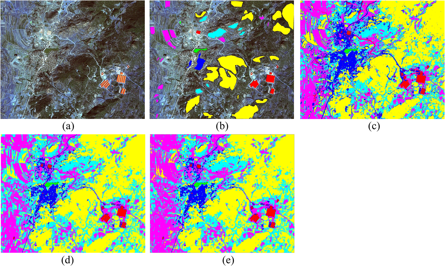

Fig. 5

Multispectral high resolution SPOT 6 image acquired over Qujing city, Yunnan province, China (sample 2). (a) RGB composition of image. (b) Ground survey of the six classes of interest identified: “industrial” (red), “water” (green), “forest” (yellow), “rock” (cyan), “arable” (magenta), and “residential” (blue). (c) ML LUC classification maps. (d) SVM LUC classification maps. (e) Fusion of SVM and FKM LUC classification maps.

It can be easily found from the labeled images that in most cases data consists of small polygons [Figs. 4(b) and 5(b)]. Much care was taken to scatter training areas across each image to ensure that they were representative of the entire image, and to retrieve as many training samples for each LUC classes (Table 1) as needed to satisfy the previously suggested criteria for establishing an appropriate minimum sample size.³¹ The Jeffries–Matusita transformed divergence index was used to assess the separability of samples data. We confirmed that separability was rather high for industrial, water, and forest, but much lower for the rock class. These pixels were all used for supervise classifiers training and validation.

Table 1

Size of LUC samples (#pixels) collected from each classification.

LUC class	Sample 1 pixels	Sample 2 pixels
Industrial	25,154	10,713
Water	5220	176,408
Forest	321,097	86,352
Rock	39,905	10,061
Arable	49,054	62,786
Residential	19,594	47,304

4.

Results

The classification maps produced by ML, SVM, fusion of FKM, and SVM classifiers are presented in Figs. 4 and 5. In Fig. 4, all classification approaches identified forest class as the LUC class occupying more than half of the total area of the zone, followed by arable class. All methods identified water class as the LUC class with the smallest area. On the contrary, the water class accounted for the largest proportion in Fig. 5.

Confusion matrices of each classification algorithm were produced to analyze classes’ separation performance. In the sample 1 image, each classifier with overall accuracy (OA) assessed at 95.4156%, 96.5497%, and 97.7760% of ML, SVM, and fusion of SVM and FKM, respectively (Table 2). The OA of ML, SVM, and fusion of SVM and FKM classifiers was 92.5530%, 96.8847%, and 97.7552% (Table 3). From both the tables, the ML classification approach created the lowest producer’s and user’s accuracies for the individual classes.

Table 2

Sample 1 LUC classification accuracy (%) of three classifiers.

Table 3

Sample 2 LUC classification accuracy (%) of three classifiers.

The sample 1 confusion matrix of fusion of FKM and SVM classification algorithm is shown in Table 4. Although the fusion of SVM and FKM classification attained highly accurate overall results, it was markedly less effective in recognizing rock and residential. About 0.43% of industrial was mistaken as residential while 1.98% of residential was wrong labeled as industrial class.

Table 4

Confusion matrixes representing best overall of classification using fusion of SVM and FKM in sample 1.

The sample 2 confusion matrix of fusion of FKM and SVM classification algorithm is also shown in Table 5. The classifier was less effective in recognizing residential to industrial or rock. About 13.31% of industrial was mistaken as residential and 14.40% of rock was wrong labeled as residential class.

Table 5

Confusion matrixes representing best overall of classification using fusion of SVM and FKM in sample 2.

5.

Discussions

ML classification map held the most details, while SVM classification map got the least particulars. It is due to SVM algorithm eventually translating into a convex optimization problem, which can guarantee the global optimal. However, ML classifier is focused on resolving the local problem and ensuring the local optimal.

Tables 2 and 3 demonstrate the SVM classifier is more effective than ML classifier in LUC classification. It is also coincided with that SVM classifier is better than ML classifier in LUC classification which was referred from many references.^47,48 Fusion of FKM and SVM classifier got the highest OA among three classifiers. The highest overall classification accuracy generated by fusion of FKM and SVM in this study suggests that our approach is useful in conducting land LUC classification.

The result was seriously influenced by the training samples because there were some shadows existing in residential and industrial training samples. The proposed method was less effective in the separation of rock and arable classes. It may be due to the date of the SPOT 6 image. The image was captured in winter. Few crops were growing on the farm in that season, so the huge area of bare soil on the farm land led to difficulty in distinguishing arable class and rock class. Because some trees or grasses grow in rock areas; and similarly, some forest areas without vegetation and bare rock turned out, the size of ground objects relative to the spatial resolution of a sensor is directly related to image variance.⁴⁹ Some errors were made between forest and rock classes. About 1.16% of rock class pixels was mistaken as forest class. About 2.06% forest and 4.86% rock were wrongly classified as residential class (Table 4), only 0.24% of forest wrongly taken as rock and 0.94% of rock mistaken as forest, which may also be caused by the residential training sample. The reasons for the big mistake distinguishing residential, industrial, and rock are as follows. First, the residential houses were smaller than the other LUC classes on the SPOT 6 image, and the residential class sample contained some trees, grasses, and naked ground. Second, there were similar buildings between the residential and industrial zones.

It can also be found that factories were built on hills and residential houses were placed near to pool from classification map, which resulted from local land use policy. Local administrators regulated to build industrial parks on the barren slopes, construct town on mountains, and develop agriculture around dams. The essence of land utilization was that the urban industrial went to the top of mountains while bottoms were exploited as farmland. This policy had brought great significance to urbanization of Yunnan province. More than 20 million hectares of mountain land were sorted out for industrial or urban use till 2012.⁵⁰

6.

Conclusion

This paper has proposed a fusion of SVM and FKM classification methods. The method can improve efficiency when dealing with remote sensing images. In this paper, the usefulness of the NDVI layer and FKM segmentation map has been demonstrated to be able to improve SVM classification in SPOT 6 images. Experiments on the SPOT 6 image classification problem showed good results, and encourage future and deep research in the field of LUC classification. To our knowledge, this is first time SVM and FKM algorithms have been combined to classify LUC. Foremost work is to focus on higher resolution images and combine more information.

Our findings are promising because accurate mapping of LUC is highly challenging over heterogeneous areas, particularly in subtropical regions, and yet this task is important to conservation initiatives, climate change mitigation strategies, and the design of management plans and rural development policies. Our classification approach presents the advantage of being easy to implement, as both the calculation of NDVI and the presence of SVM classifier are readily available in remote sensing software and cost-effective, as SVM classifiers may use smaller training data sets without compromising classification accuracy. Importantly, the highly accurate results obtained by this approach suggest its great potential for LUC mapping in subtropical areas. We will assess in other areas in the near future.