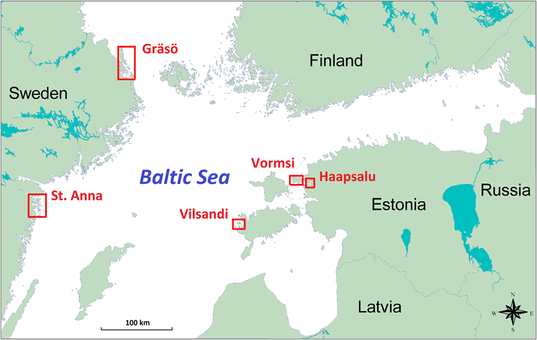
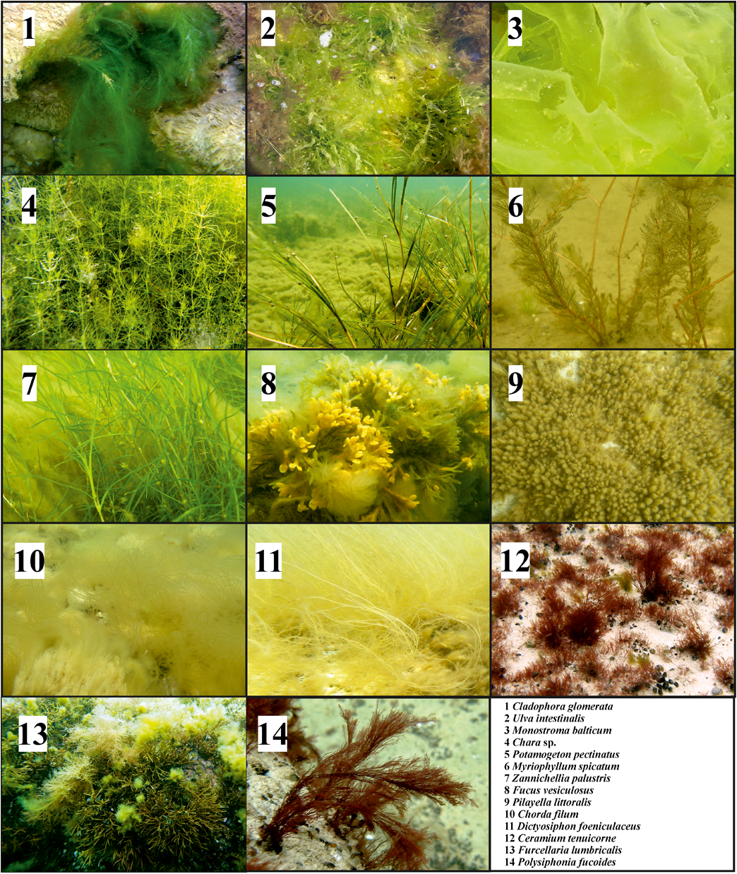
1.

Introduction

Marine macrophyte communities have high ecological and economic importance. They form extensive habitats in near-coastal zones and are among the most productive habitats worldwide. Consequently, they provide a range of ecological functions, such as protecting coastlines, stabilizing sediments, attenuating waves, filtering land-derived nutrients, and binding carbon, just to name a few. Nowadays, the patterns of species composition of marine macrophytes are used to assess the state of coastal marine environments in sensu according to the EU Water Framework Directive and the EU Marine Strategy Framework Directive. Although the Marine Strategy Framework Directive require a seamless quantification of the cover of macrophyte beds over a range of seascapes, to date, the vast majority of studies have been performed on limited spatial scales, i.e., the size of sampling units remained small and vast areas between grains were left unstudied.^1,2 Therefore, there is a strong need for methods that allow collecting qualitative and quantitative information about these shallow-water benthic habitats over large sea areas.

The use of remote sensing for improving ecological understanding, monitoring, and managing of marine coastal areas has certain advantages: the method permits synoptic mapping of large areas, allows mapping of inaccessible zones, and is often more cost-effective than conventional methods, e.g., diving and grab sampling.^3,4 Many macrophyte species potentially have distinctive spectral signatures detectable using remote sensing. In order to map the spatial distribution of these species, their spectral properties have to be quantified.

A basic assumption of mapping by remote sensing is that the features of interest in an image reflect or emit light energy in different and often unique ways.⁵ Thus, only the spectrally different features can be mapped. The spectral signatures of submerged benthic vegetation are principally determined by their pigment composition. Earlier studies have demonstrated spectral dissimilarities between the three major groups of macroalgae—the green, brown, and red algae.^6–9 All these macroalgae contain chlorophyll a, but differ in the presence of other chlorophylls and accessory pigments, such as carotenoids (carotenes, xanthophylls) and phycobilins (phycocyanin, phycoerythrin).¹⁰ Nevertheless, it is also plausible that within these broad taxonomic groups, many macroalgal species have unique pigment combinations.

Spectral signatures are one of the most promising features of coastal aquatic systems that can be exploited for both science and management applications of remote sensing.^11–13 In such a spectral library approach, remote sensing reflectance spectra (Rrs) of individual pixels in the images are compared to measured/simulated Rrs spectra.^12,14 Creating a modeled spectral library requires measured values of bottom reflectance and data about inherent optical water properties.¹⁴ The advantages of spectral library approach are that there is no need of extensive field surveys¹² when the optical properties of benthic habitats are determined and possible variability in optical water properties can be estimated. There is no need to collect in situ data simultaneously at the time of image acquisition; it is easy to apply the methodology on data from different sensors as the spectral library can be recalculated for spectral bands of each sensor. There is also no need of depth data as the method resolves both depth and benthic habitat type information simultaneously. However, high-quality atmospheric correction is required to classify a remote sensing image using a modeled spectral library.

The spectral library approach requires a quantification of the range of signatures expected for any species under natural conditions.^14–17 In nature, however, there exists a considerable variation in pigment composition and quantity among broad taxonomic groups and even within species. For example, the brown algae may range in color from beige to almost black.¹⁸ Such differences may be related to species-specific character of pigment composition but also induced by environmental factors, such as light, nutrients, and water flow.¹⁰ Moreover, the overall spectral appearance of an alga cannot necessarily be inferred based only on the knowledge of the pigments present. The morphology, thickness of thalli, and cellular architecture affect the relationship between pigment densities and absorption spectra^19–21 and, consequently, affect the formation of reflectance spectrum. At the other extreme, however, some authors have questioned whether spectral signatures of individual plants are unique at all.¹⁵ This plethora of diversity makes it very challenging to establish the typical ranges of reflectance spectra of macrophyte species and assess significant differences among groups. To date, spectral signatures of the ecological end-members have been published for some corals, macroalgae, and seagrasses.^{9,18,22,23–25} Nevertheless, these studies mainly concentrated on species growing in ocean waters. Moreover, very few did account for the variability of spectral signal within and between species (e.g., Ref. 22). To assess a potential of remote sensing methods for monitoring macrophyte beds, however, ranges of spectral signal of macrophyte need to be quantified, and spectral regions that consistently allow discrimination of species or taxa need to be defined.

The development of tools that allow distinguishing the reflectance spectra of different species is often complicated by nonstandardness. Such variability largely degrades the performance of any image processing tool. Standardizing may refer to many types of ratios, but usually this is done by subtracting the mean of the particular spectrum from the raw reflectance values and dividing by the standard deviation of the same raw reflectance values. Usually standardization refers to a preprocessing step that aims to improve reflectance constancy by realigning intensity distributions of images. However, a standardization algorithm can as well be applied for reflectance spectra, i.e., instead of preprocessing pixels of images, reflectance values at different wavelengths are corrected by the properties of spectral signature over the whole spectral range.

Based on the above, the objectives of this study were (1) to quantify the spectral properties and variability of the key benthic macrophyte species in the Baltic Sea area; (2) to demonstrate a methodology that allows quantification of statistical differences between the reflectance spectra of macrophyte species and broad taxa by utilizing both nonstandardized and standardized spectra; and (3) to define which spectral regions contribute most to the observed statistical differences.

2.

Material and Methods

2.1.

Study Area

The Baltic Sea is an intracontinental shallow marine environment under a strong influence of human activities and terrestrial material. Large discharge from rivers, limited exchange with marine waters of the North Sea, and extensive shallow areas significantly influence the optical properties of the Baltic Sea.²⁶

The Baltic Sea hosts all three main groups of macroalgae (green, brown, and red macroalgae) as well as higher plants. In this study, an array of macroalgae and higher plant species were collected from the Estonian and Swedish waters (Fig. 1). The Vilsandi National Park is located in the western coast of Saaremaa Island and it encompasses $\sim 160$ islands and islets of different sizes. Most of the area is $<5\mathrm{m}$ deep although in a few locations water depth reaches 15 m. Haapsalu Bay extends deeply into the land in the western part of Estonia. The bay is relatively shallow with an average depth of 1.5 to 2 m and a maximum of 5 m. Vormsi Island is located west of the Estonian mainland. Most of the study areas were $<5\mathrm{m}$ deep. The island has extensive shallows in the southern parts and steep and more exposed coasts in its northern parts. Gräsö Island and the St. Anna archipelago are characterized by thousands of islets and bays. Water is generally $>10\mathrm{m}$ deep, i.e., the bottom signal is not detectable by remote sensing sensors. Shallow areas occur only near coast and in small bays and channels between islets.

Fig. 1

Macrophyte sampling sites in the Baltic Sea.

2.2.

Field Survey

Altogether 531 taxa of benthic vegetation have been found in the Baltic Sea.²⁷ It would be excessively labor-intensive to collect reflectance spectra for each of these species.²⁸ Moreover, such a task would not be rational since a large number of taxa are rare, hidden in crevices, or spatially imbricate over a few square centimeters.²⁴ Moreover, due to similar pigmentation, the reflectance spectra are likely similar for many of these species. Therefore, only the key macroalgae and higher plants were collected for reflectance measurement. The samples included the green algae Cladophora glomerata, Ulva intestinalis, Chara spp., Monostroma balticum; the higher plants Potamogeton pectinatus, Myriophyllum spicatum, Zannichellia palustris; the red algae Ceramium tenuicorne, Furcellaria lumbricalis, Polysiphonia fucoides; and the brown algae Fucus vesiculosus, Pilayella littoralis, Chorda filum, and Dictyosiphon foeniculaceus (Fig. 2). In addition, reflectance spectra of bare sand, pebble, limestone, and silt were measured on different beaches.

Fig. 2

Still photographs of the studied macrophyte species.

Water molecules absorb light strongly in red to near-infrared part of the spectrum, i.e., in the part of spectrum where the main differences between different benthic species occur.²⁹ Just a few centimeters of water between the sample and the sensor affect the measured reflectance significantly. Determining the accurate distance between the sample and sensor is not practically possible during in situ measurements as the water depth, where the measurements have to be carried out, varies between a few centimeters to $\sim 10\mathrm{m}$ in the Baltic Sea. Therefore, obtaining the true reflectance of different algae and plants without any impact of water column by means of in situ measurements is practically impossible. Nevertheless, unlike terrestrial vegetation,^30,31 leaf orientation and canopy geometry are not coupled with the reflectance spectra of aquatic vegetation. Such specific characteristic of macrophytes is an unavoidable consequence of the evergoing mobility of aquatic organisms under the wave exposure. Our long experience in carrying out reflectance measurements in shallow waters suggests that differences in the geometry of canopy do not practically change reflectance spectra, and variation in the canopy properties only marginally contributes to the absolute reflectance values. These changes are likely smaller than the potential uncertainties due to unrecorded distance between the sample and the sensor. Our pilot study also indicated that only slight changes in true reflectance are expected if the macrophytes are removed from water (Fig. 3).

Fig. 3

A comparison of raw (a, b) and standardized spectra (c, d) of Fucus vesiculosus (a, c) and Pilayella littoralis (b, d) in water and in air. The standardization was done by subtracting the mean of the particular spectrum from the raw reflectance values and dividing by the standard deviation of the same spectrum.

Due to the above-mentioned considerations, macrophytes were taken out from the water, placed on a black plastic bag as piles, and then their reflectance spectra were immediately measured with Ramses hyperspectral radiometers, built by TriOS GmbH (Germany). The macrophytes were kept wet during the measurements. The plastic was mainly used to minimize signal from the adjacent environment. However, the measurements were done in a way that no plastic was seen by the sensor. Five to ten individual spectra were measured for each specimen. The measurements were performed over the entire plants and not only over the blades of the plants in order to cover possible spectral variability within each specimen. Measurements were conducted in the visible and near-infrared range of the spectrum (350 to 900 nm) with $\sim 3\text{-}\mathrm{nm}$ spectral interval. Downwelling light was measured by irradiance sensor and upwelling light by radiance sensor above the sample. In most cases, we used a standard Trios cage while some measurements were carried out holding upwelling radiance sensor by hand. This was needed in order to be able to measure reflectance of different parts of specimens that had more complex canopy structure and visible differences between different parts of the canopy (for example, in the case of Fucus vesiculosus). In order to determine the reflectance spectra of each sample, the upwelling radiance (Lu) was divided by the downwelling irradiance (Ed).

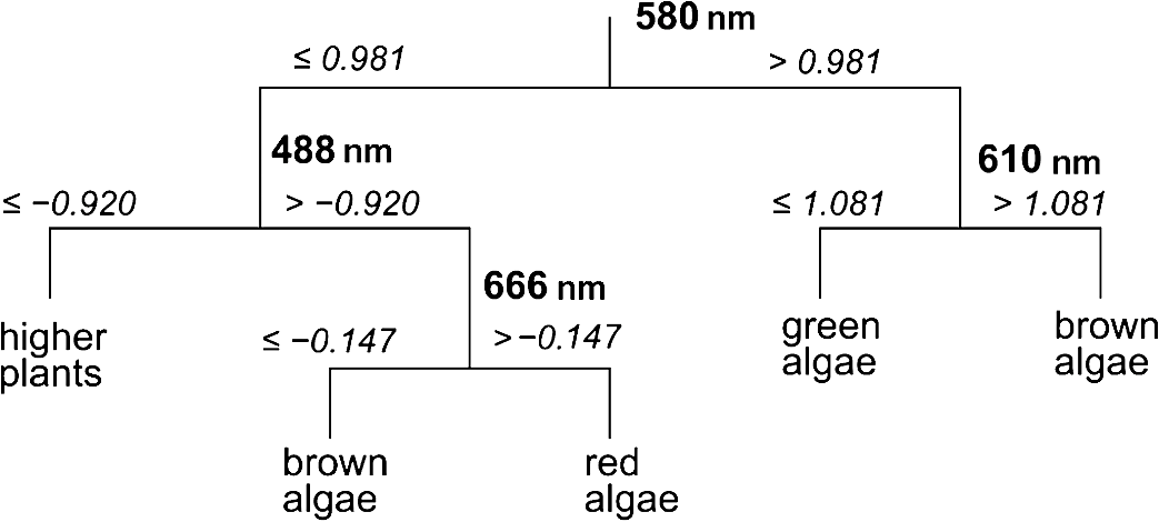
3.

Results

Among green macroalgae, Ulva intestinalis was the brightest species with the highest reflectance values. Ulva was followed by Monostroma balticum, Cladophora glomerata, and Chara spp. All green algal species showed a broad reflectance peak centered at 550 nm and reflectance trough around 675 nm, which corresponds to the chlorophyll absorption peak [Fig. 4(a)]. Brown algal species had consistent shape in their reflectance spectra, i.e., reflectance peaks at 600 and 650 nm and a shoulder at 580 m; however, the absolute reflectance values varied among species. Dictyosiphon foeniculaceus showed the highest reflectance, reaching 4.5% in the visible part of the spectrum. The reflectance values of dark brown Fucus vesiculosus reached only 1% in the visible part of the spectrum. Red algae had two clear reflectance peaks at 600 and 650 nm. Furcellaria lumbricalis was darker than Ceramium tenuicorne and Polysiphonia fucoides, showing the lowest reflectance value throughout the entire spectrum of the red algae. Higher plant species had no specific spectral features of raw reflectances but a high reflectivity over a broad wavelength range (550 to 640 nm). However, a standardization of the reflectance spectra resulted in relative high reflectances at 675 nm.

Fig. 4

The reflectance values of the studied plant individuals: (a) raw data and (b) standardized data.

The raw reflectance spectra of plant individuals were largely overlapping and did not enable a reliable distinction of species and larger taxonomic groups [Fig. 4(a)]. The standardization led to considerable improvement, first of all in the distinctness of green algae compared to the group of brown and red algae [Fig. 4(b)]. The green algae had higher standardized reflectance values in the spectral range of 510 to 582 nm, which corresponds approximately to the visible green light. In most other spectral regions, the reflectance of red and brown algae exceeded the values of green algae (recall that the mean of a standardized sample is always equal to zero).

The results of Kruskal-Wallis tests also indicated that difference in the distribution of standardized reflectance values of a particular spectral interval between broad taxonomic groups is statistically significant ($p<0.05$) in most spectral intervals, while the raw values differ significantly only within a narrow spectral range between 530 and 580 nm. The best indicative spectral range was observed between 530 and 570 nm if both species and larger taxonomic units were considered. In general, difference between broad taxa was more significant than that of the studied species (Fig. 5).

Fig. 5

Statistical significance ($p$) according to the Kruskal-Wallis test of the difference in reflectance values between the studied groups of plant individuals. Solid lines refer to raw signatures and broken lines to standardized signatures.

Statistically significant, i.e., reliably not random, distinction between the major taxonomic groups in our data is possible at certain spectral ranges only (Fig. 6). Distinction values in standardized reflectance spectra were found even for the generally similar red and brown algae. According to our sample, a classification result, which is significantly better than expected from random decisions, is possible at 558 to 582 nm. On average, the wavelength intervals at 470 to 492, 520 to 582, 646 to 658, and 670 to 680 seem to be most indicative to distinguish broader taxonomic groups of macrophytes, although the distinction is perfect only in case of some intervals and between some groups, e.g., green and brown algae at 530 to 560 nm.

Fig. 6

Statistically significant distinction lines (thick black line) between the standardized signatures of broad taxonomic units of benthic macrophytes (above) and the true skill statistic (TSS) (below) when imposing the distinction values upon the studied sample. $\mathrm{TSS}=1$ means perfect distinction in the study sample. Distinction line is depicted in spectral regions where the classes differ significantly according to the U-test.

Although the differences between distribution spectral values are mostly statistical and not perfect, there still exist a set of rules enabling perfect separation of broad taxonomic groups in our sample (Fig. 7). Variability outside the study sample is expected to be much larger.

Fig. 7

Classification tree for separating broad taxonomic units of benthic macrophytes using standardized spectral values. Bold numbers mark wavelength in nanometers, and critical values for decisions are in italics.

4.

Discussion

The current paper is the first comprehensive investigation on the measured reflectance spectra of the key macrophyte species in the Baltic Sea. These spectra can now serve as key inputs to the spectral library approach in order to map the spatial and temporal patterns of coastal macrovegetation in the Baltic Sea range. Although the measurements showed some clear-cut differences between some macrophyte species, many species had still very similar reflectance values.

We also demonstrate a methodology that allows a statistically significant separation of spectral signatures of different macrophyte species and broader taxonomic groups. In remote sensing, a spectrum of macrophyte species is often defined as a static object, i.e., the values are averaged over space and time.^23–25 However, in nature, there exists a considerable variation in the composition and quantity of pigments within species induced by seasonality in light conditions, nutrient availability, exposure to waves, just to name a few (e.g., Ref. 4). Thus, it becomes rewarding and ecologically meaningful to quantify spatiotemporal variability in reflectance within species/taxa and then seek statistical options for species separation taking into account all this natural variability.

Our analyses showed that the shapes of reflectance spectra of red, green, and brown macroalgae were consistent within each group due to the presence of characteristic pigments,^8,25 and the separation of these broad groups of algae by a shape of their reflectance spectra was possible. Specifically, green algae had high reflectance in the green part of the spectrum from 500 to 650 nm with the highest reflectance centered at 550 nm. Characteristic green algal pigments—chlorophyll a, chlorophyll b, and $\beta$-carotene—absorb strongly in the blue and red part of the spectrum. The presence of those absorbing pigments provokes low values in the bands from 400 to 500 nm as well as from 650 to 680 nm. Chlorophyll a has absorption peaks at $\sim 435$ and 675 nm,³⁸ chlorophyll b absorbs at $\sim 480$ and 650 nm (Ref. 27), and $\beta$-carotene at $\sim 425$, 451, and 483 nm.^39,40

The brown and red macroalgae had distinctly different signatures from one another and from the green algae. Once again, a distinct absorption maximum near 675 nm is conditioned by chlorophyll a absorption. Compared to green algae, the maximum reflectance values for brown macroalgae were located at the 570- to 650-nm wavelengths. Brown algae showed enhanced absorption at the 500- to 550-nm spectral region due to fucoxanthin absorption.⁴¹ Another characteristic pigment for brown algae is chlorophyll c, which absorbs around 460 and 633 nm.²⁸ The shape of the brown algae reflectance spectra is analogous to other brown algae and many corals (containing symbiotic brown algae) measured in different parts of the world.^17,25 The brown algae in the Baltic Sea showed broad reflectance peaks at 570, 600, and 650 nm corresponding to previous measurements in the world seas.^6,7,9,12,42

Red algae were discernible from other algal groups by the presence of a dip in reflectance at 570 nm.¹⁰ In addition to chlorophyll a and carotenoids, the characteristic pigment in red algae is phycoerythrin.³⁸ Characteristic chlorophyll a absorption maxima were seen at 435 and 675 nm just as in case of green and brown macroalgae. Low reflectance values appearing in shorter wavelengths from 400 to 500 nm were conditioned by pigments $\beta$-carotene and $\alpha$-carotene.⁴³ Phycoerythrin absorbs strongly in the middle of the visible spectrum with absorption peaks near 495, 540, and 565 nm, depressing reflectance values in the green part of the spectrum and is, thus, almost complementary to chlorophyll in its absorption.³⁸ The presence of chlorophyll c was also detectable by a small shoulder near 630 nm.⁴³ The red algae had a common double-peak pattern around 600 and 650 nm in their reflectance spectra, all this resembling the studies performed in other parts of the world.^6,7,12,42

When raw reflectance values were considered, the variability within each broad taxonomic group was large and a statistical separation even among the broad macrophyte taxa was difficult. This is because the shapes of reflectance spectra of macrophyte species and taxa highly resemble each other due to the similar pigment content and overlapping absorption features of biochemical constituents. Standardized spectra partly resolved the issue; however, the separation of species still posed a great challenge. Nevertheless, a standardization of reflectance spectra was useful as it reduced noise due to natural variability of the pigment composition of macrophytes.

Statistical discrimination models used in image preprocessing (both parametric and nonparametric) need many samples in order to be trained and evaluated. However, the collection of large numbers of samples is not normally feasible, and thereby, the traditional image-based analyses do not yield to accurate discrimination models. On the other hand, the spectral library approach requires much smaller data sets and, in case of availability of high-quality atmospheric correction, the method allows an efficient mapping of benthic macrophyte communities over a large spatiotemporal range. Nevertheless, the existing spectral libraries often consist of averaged reflectance values, ignoring spectral variability among individual and taxa. In order to quantify ranges of variability, however, more empirical data are needed. Instead of providing just average species-specific reflectances, the raw values (i.e., separate measurements of each individual) are of utmost importance. When such information is available, it becomes rewarding to seek the optimal separating boundary between the taxa based on their statistical separation. Then, this information is used to define a set of rules enabling perfect separation of the studied taxa. Those rules represent the distinct parts of reflectance spectra where the overlap between the taxa is statistically the smallest.

In the proposed method, the original observed spectra are standardized by subtracting the mean of the spectral signature from spectral values and dividing the result by the standard deviation of values within the spectrum of a plant individual. Then, the TSS is applied as a decision basis to find the optimal separating boundary between the taxa, assuming that the best separating boundary between the taxa should be between medians of the values of one and another sample. The boundary can separate two samples either perfectly or statistically. The statistical separation can be significant or nonsignificant according to a chance of Type 1 statistical error bound with the analysis.

Unfortunately, the optimal boundaries between all possible pairs of taxa are not easy to be used for determination of a taxon from a remote sensing data. For recognition of categories, we need rules on how to use similarity, separating values, or any other decision criteria. The option to use similarity-based or case-based reasoning is effective, first of all, if the cases are complicated, the number of variables is large, different types of variables are included, and the number of cases is enormous and continuously increasing.^44,45 For the present simpler case, we preferred building a hierarchical set of rules as a CART model for recognizing the taxa from remote sensing spectra. Such a classification tree enabled a perfect separation of the broad taxa in our data. The CART algorithm has been widely used to obtain an adequate set of rules allowing the separation of various end-members.^46,47 Similarly, in our study, we extracted the most rewarding features for the discrimination of the studied macrophyte taxa. The key idea behind the method is that it is difficult to separate taxa by relying only on one classifier computed at a single wavelength. In addition, the CART analysis reduces the number of statistically significant bands selected by the Kruskal-Wallis test and by the Mann-Whitney U test to fewer bands that could optimally discriminate the macrophyte taxa under concern. It is still useful to preselect and include only these spectral ranges where the separation between the taxa is significant according to the statistical tests, since the CART-based methods may be quite sensitive to data noise.⁴⁸

We are fully aware that the current database consists of too few estimates at the species level. Nevertheless, the presented methodology allows establishment of the robust criteria in order to separate (at least some) macrophyte species in the Baltic Sea range if one increases the number of macroalgal individuals used in the training data set and if the distinct spectral features used to draw the borderline among species are maximized. Specifically, with an increasing number of rules, the probability of discriminating macrophyte species notably increases. This result encourages further evaluation of the methodology over a larger number of species.

In simple environments, including the Baltic Sea basin, macrophyte communities consist of limited numbers of species, and each broad taxon (e.g., green, brown, and red algae) is often represented by single species.^13,49 In such habitats, it is already satisfying to separate only broad taxonomic groups in order to recapture the spatial distribution of coastal macrophyte communities. However, in more complex environments where biodiversity is higher and each species is characterized by a large natural within-species variability in reflectance spectra either due to genetic variation, seasonal cycles, or environmental conditions,^43,50 mapping the macrophyte communities at the species level may be impossible. To conclude, the potential of the spectral library approach depends, on one hand, on the representativeness of training data set and, on another hand, on the habitat complexity and associated biodiversity. The question remains, still, how to discern species from multispecies assemblages using the spectral library classification approach. In such complex habitats, macrophytes do not grow as monospecific stand but occur in mixtures. The mixed assemblages are likely characterized by reflectances that are not necessarily the sums of the reflectance spectra of individual species. Therefore, we need to evaluate the validity of spectral standardization in future work by focusing on the reflectance spectra of mixed assemblages.