Derivation and approximation of soil isoline equations in the red–near-infrared reflectance subspace

Kenta Taniguchi; Kenta Obata; Hiroki Yoshioka

doi:10.1117/1.JRS.8.083621

3 June 2014 Derivation and approximation of soil isoline equations in the red–near-infrared reflectance subspace

Kenta Taniguchi, Kenta Obata, Hiroki Yoshioka

Author Affiliations +

Journal of Applied Remote Sensing, Vol. 8, Issue 1, 083621 (June 2014). https://doi.org/10.1117/1.JRS.8.083621

Abstract

This study describes the derivation of an expression for the relationship between red and near-infrared reflectances, called soil isolines, as an orthogonal concept for the vegetation isoline. An analytical representation of soil isoline would be useful for estimating soil optical properties. Soil isolines often contain a singular point on a dark soil background. Singularities are difficult to model using simple polynomial forms. This difficulty was circumvented in this work by rotating the original axis and employing a vegetation index-like parasite parameter. This approach produced a soil isoline model that could yield any desired level of accuracy based on the use of an index-like parameter. A technique is further introduced for approximating the removal of the parasite parameter from the relationship by truncating the higher-order terms during the derivation steps. Numerical experiments by PROSAIL were conducted to investigate the influence of the truncation errors on the accuracy of the approximated soil isoline equation. The numerical results showed that truncating terms of order greater than two in both bands, yielded negligible truncation errors. These results suggest that the derived and approximated soil isoline equations may be useful in other applications, such as the analysis and retrieval of soil optical properties.

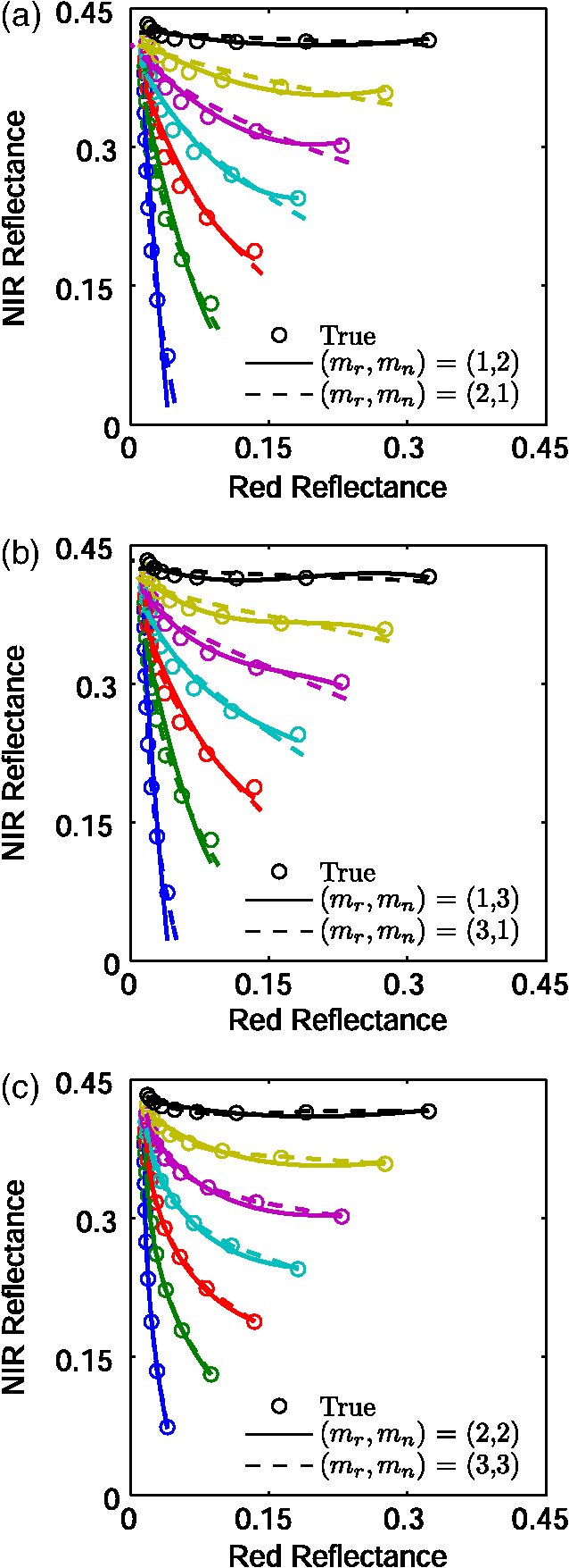
1. Introduction

Parameter retrieval algorithms based on remotely sensed land surface reflectance data often involve band algebraic manipulations and produce environmental data records, such as vegetation biophysical parameters or soil optical properties. Some algorithms use an intermediate proximity measure, e.g., the spectral vegetation index (VI), either explicitly or implicitly.¹^–⁵ The performances of the data records depend somewhat on the functional forms of VIs; hence, research in this field has extensively explored the development and improvement of functional forms over the last few decades.¹^,²^,⁶^–¹¹ Numerous VI models have been developed through these efforts.¹^,¹²^–²¹

VI models may be categorized systematically according to the concept of the isoline used to develop and analyze the VI.⁷^–⁹^,¹¹^,²²^–²⁸ Limiting our discussion to VI models of the red and near-infrared (NIR) reflectance space, two main types of isolines have been recognized: the vegetation index isoline (VI isoline) and the vegetation biophysical isoline (the latter is denoted as vegetation isoline in this study).¹^,⁹^,¹¹^,²²^,²³^,²⁶^,²⁸ The VI isoline represents a set of red and NIR reflectance spectra that produce a single VI value, meaning that the VI isoline depends only on the VI model equation. This point is illustrated in Fig. 1(a) using the normalized difference VI as an example. The vegetation isoline [Fig. 1(b)], on the other hand, describes a group of reflectance spectra that belongs to a fixed set of biophysical parameters and structural properties, such as the leaf area index (LAI), fraction of vegetation cover (FVC), and leaf angle distribution. The vegetation isoline can be simulated numerically using a radiative transfer model of the vegetation canopy.²⁹^–³² Note that these two isolines (VI isoline and vegetation isoline) have no physical relationship, meaning that the two are obtained independently. Also, note that the ultimate goal of the VI development effort may be understood as an effort to identify a VI model equation that yields VI isolines that agree perfectly with the vegetation isolines.¹^,⁹^,¹¹^,²²^,²³^,²⁶^,²⁸ Several studies suggest that the discrepancies between the VI isoline and the vegetation isoline indicate performance losses in the VI model as a result of internal and external sources of errors, including the influence of soil brightness changes beneath the vegetation canopy.¹¹^,¹⁸^,¹⁹^,²⁵^,³³^–³⁷

Fig. 1

Illustration of the vegetation index isolines (a), vegetation biophysical isolines (b), and soil isolines (c). The concept of the soil line is illustrated in (b), and (c) illustrates a zero vegetation isoline.

Formulations of the vegetation isoline have been developed in several previous studies.¹^,¹¹^,²²^,²³^,²⁶ These formulations have been used to develop VI models and analyze VI errors.¹^,¹²^–²¹ The isoline equations have been used directly to retrieve the LAI (Ref. 38) and FVC (Ref. 39) from a remote sensing data set. In recent years, the isoline equation, which describes the relationship between the red and NIR reflectances, has been used to cross-calibrate the VI products obtained from multiple sensors.²⁵^,⁴⁰^–⁴⁴ These activities clearly indicate that the concept of the isoline has provided rich information and useful tools for a variety of investigations. The concept of the isoline has significantly advanced research in this field.

The concept of the isoline is not limited to biophysical properties. An alternative to the vegetation isoline is the soil isoline, which represents a group of reflectance spectra produced from a constant soil surface. Note that a soil isoline is totally different from the concept of the soil line,²⁷ which is a zero vegetation isoline. In other words, the soil line is a vegetation isoline describing the particular case of zero vegetation, whereas the soil isoline is a set of spectra obtained under a constant set of soil reflectance spectra, in view of various biophysical parameters. This point is illustrated in Fig. 1(c).

Extensive efforts have been devoted toward studies of vegetation isolines; however, soil isolines have not been fully investigated. The present study aims to contribute to this area of research. Singularities at relatively dark soil surfaces present a significant barrier to modeling soil isolines using a simple polynomial form.¹⁰ Limiting our discussion to the red–NIR reflectance space, under low levels of soil reflectance, the soil isoline becomes approximately parallel to the NIR axis. As a result, some of the polynomial coefficients become extremely large. Such singularities must be circumvented in any soil isoline model. A numerical example of this situation is discussed in the next section.

The concept of the soil isoline is not new. Soil isolines have been introduced and routinely used as a conceptual tool on various occasions to explain band manipulation algorithms and their performances in the presence of external sources of errors.¹^,⁹^,⁴⁵^,⁴⁶^,⁴⁶^–⁵² The concepts have not been fully investigated, however, nor have they been developed analytically to date. Formal derivations of soil isoline estimation algorithms and the accuracy of such approaches when applied to truncated higher-order terms must be explored in anticipation of soil isoline applications. This study attempts to address these needs.

Three objectives have guided this study. First, we introduce a formal derivation of soil isoline equations that give an arbitrary level of accuracy. Second, we describe a technique for approximating the analytical representation. This approximation is more amenable to applications than the analytical expression. Finally, we characterize the accuracy of the approximated form of the soil isoline equations. A set of numerical experiments were carried out using a canopy radiative transfer model to estimate the model accuracy. This work is an extension of our previous studies, described elsewhere.⁴⁷^,⁴⁸

2. Difficulty in Modeling Soil Isolines Using Polynomial Fitting Approaches

The difficulties associated with modeling soil isolines are briefly mentioned above. Here, we describe an illustrative numerical example of a soil isoline modeled using a second-order polynomial. In this model, the soil isoline is expressed in terms of the relationship between the red ( $ρ_{r}$ ) and NIR ( $ρ_{n}$ ) reflectances according to

Eq. (1)

ρ_{n} \approx k_{0} (R_{s}) + k_{1} (R_{s}) ρ_{r} + k_{2} (R_{s}) ρ_{r}^{2},

where

k_{0}

,

k_{1}

, and

k_{2}

represent the polynomial coefficients.

A reflectance spectrum ( $ρ_{r}$ , $ρ_{n}$ ) may be numerically simulated using the radiative transfer model PROSAIL.³¹ During the simulation, only two parameters are varied: LAI and the soil reflectance of the red band $R_{s}$ . Because we assumed a soil line, the soil reflectance of the NIR band was uniquely determined based on the soil line equation from the red reflectance $R_{s}$ . For this reason, we did not explicitly introduce the NIR reflectance of the soil surface in this study. An isoline was numerically simulated by setting the soil reflectance $R_{s}$ to a fixed value, meaning that the LAI was the only variable parameter used to optimize each soil isoline in this example. After simulating each soil isoline (under a constant value of $R_{s}$ ), a set of three coefficients ( $k_{0}$ , $k_{1}$ , and $k_{2}$ ) was obtained through polynomial fitting approaches. These steps were repeated for various values of $R_{s}$ to obtain the coefficients $k_{i}$ as a function of $R_{s}$ . Figure 2 shows a plot of the coefficients $k_{i}$ as a function of $R_{s}$ . As shown in the figure, the coefficient $k_{2}$ assumed an extremely high value at low values of $R_{s}$ , which prevented the development of accurate polynomial models. These difficulties arose from the fact that some soil isolines in dark soils are almost parallel to the NIR axis. The reflectance axis may be rotated through an angle to circumvent these difficulties. The next section provides a stepwise derivation of the soil isoline equation that avoids these difficulties.

Fig. 2

Variations of the polynomial coefficients $k_{0}$ , $k_{1}$ , and $k_{2}$ used to approximate soil isolines in the red and near-infrared (NIR) reflectance space. Each soil isoline was simulated for a fixed soil reflectance $R_{s}$ . The coefficients were then obtained numerically from a polynomial fit of the simulated soil isolines. The coefficients as a function of $R_{s}$ are plotted in the figure. Note that the coefficients $k_{2}$ approached extremely high values, indicating the presence of a singularity at low values of 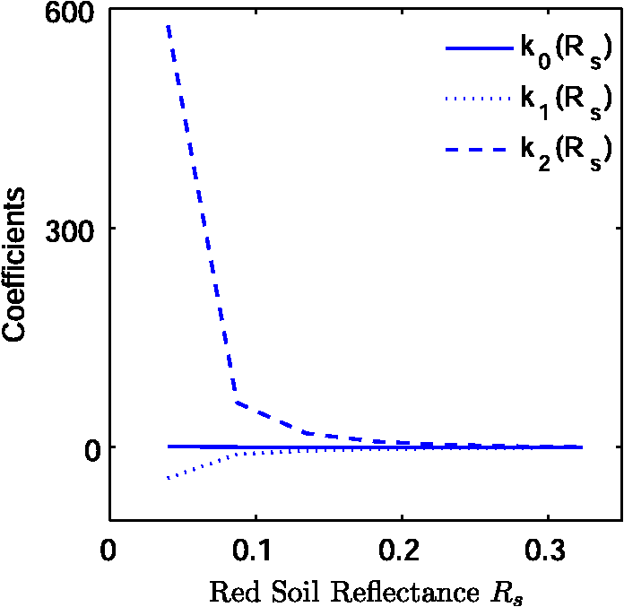$R_{s}$ .

3. Parametric Representation of the Soil Isoline Equation

3.1.

Assumptions and Transformation

The derivation begins with the assumption of a linear soil line represented by

Eq. (2)

R_{sn} = s_{1} R_{sr} + s_{0},

where

s_{1}

and

s_{0}

are the slope and offset, respectively.

In our derivation of the soil isoline equation, the original reflectance subspace was shifted and rotated through a certain angle to avoid the singularity shown in Fig. 2. The original coordinate was shifted to set the intersection between the $Y$ axis and the soil line to be the origin of the transformed subspace. The rotation angle was identical to the slope of the soil line ( $θ$ in radians). The transformation may be expressed as

Eq. (3)

ρ^{'} = T (- θ) (ρ - μ),

where

T

represents a rotation matrix,

ρ

and

ρ^{'}

are the reflectance spectra before and after the transformation, respectively, in the red and NIR reflectance space.

Eq. (4)

ρ = {(ρ_{r}, ρ_{n})}^{t},

Eq. (5)

ρ^{'} = {(ρ_{r}^{'}, ρ_{n}^{'})}^{t} .

The vector $μ$ shifts the $X$ axis by an amount equal to the soil line offset.

Eq. (6)

μ = {(0, s_{0})}^{t} .

Because the axis is rotated through an angle between the soil line and the $X$ axis, $θ$ is defined by the soil line slope $s_{1}$ as

Eq. (7)

θ = \tan^{- 1} (s_{1}) (- π / 2 < θ < π / 2) .

Finally, the relationships between the reflectances before and after the transformation become

Eq. (8)

ρ_{r}^{'} = \cos (θ) ρ_{r} + \sin (θ) (ρ_{n} - s_{0}),

and

Eq. (9)

ρ_{n}^{'} = - \sin (θ) ρ_{r} + \cos (θ) (ρ_{n} - s_{0}) .

The NIR reflectance in the transformed reflectance space, Eq. (9), plays an important role in this study. The NIR reflectance assumes a form similar to that of a VI known as the weighted difference vegetation index (WDVI).¹⁴ This result may be understood by rearranging Eq. (9) to give

Eq. (10)

ρ_{n}^{'} = \cos (θ) (ρ_{n} - s_{1} ρ_{r} - s_{0}) .

This model and the WDVI model are distinguished by the factor $\cos (θ)$ and the offset $- s_{0}$ . Because both the factor and the offset are constant values, the functional behavior of $ρ_{n}^{'}$ is essentially identical to that of WDVI ( $V$ ), which is defined as

Eq. (11)

V = ρ_{n} - s_{1} ρ_{r} .

This study used $ρ_{n}^{'}$ as a parasite parameter during the derivation of the soil isoline equation. The parasite parameter yielded behavior indistinguishable from that of WDVI, and the soil isoline equation was expected to be strongly correlated with biophysical parameters, such as LAI. The validity of the choice of this parameter may be understood intuitively by recalling that a major source of variation in the soil isoline is the biophysical parameters. (A soil isoline is obtained under conditions of a fixed soil profile.)

3.2.

Polynomial Model in the New Reflectance Space

Our next step of the derivation involved modeling the relationship between $ρ_{r}^{'}$ and $ρ_{n}^{'}$ (Fig. 3). A simple polynomial representation was used for this purpose. $ρ_{r}^{'}$ was modeled using a power series of $ρ_{n}^{'}$ .

Eq. (12)

ρ_{r}^{'} = \sum_{i = 0}^{m_{p}} p_{i} (R_{s}) ρ_{n}^{' i} + O (ρ_{n}^{' m_{p} + 1}),

where

m_{p}

and

p_{i}

represent the order of the polynomial and the coefficients of the

i

’th-order term.

R_{s}

indicates the soil reflectance. This relationship may be approximated to an arbitrary order of accuracy by selecting a polynomial based on an orthogonal set of functions, such as the Chebyshev polynomials. Therefore, this part of the modeling process did not deteriorate the accuracy of the model. The first term on the right-hand side of Eq. (12) is defined as the function

f_{m_{p}} (R_{s}, ρ_{n}^{'})

and will be discussed further later in this study.

Eq. (13)

f_{m_{p}} (R_{s}, ρ_{n}^{'}) = \sum_{i = 0}^{m_{p}} p_{i} (R_{s}) ρ_{n}^{' i} .

Fig. 3

Illustration of the soil isolines obtained after applying a space transformation to fit the original red axis to the soil line. The $x$ and $y$ axis were identified with $ρ_{n}^{'}$ and $ρ_{r}^{'}$ , respectively. Upper lines correspond to soil isolines at brighter soil.

We were interested in examining the variations in $p_{i}$ as a function of the soil reflectance $R_{s}$ . The parameter $p_{i}$ varied smoothly over a small range of values, unlike the polynomial fit results obtained from the original reflectance space, as described in Fig. 2. The coefficients $p_{i}$ were obtained numerically by assuming a second-order polynomial.

Eq. (14)

ρ_{r}^{'} \approx p_{0} (R_{s}) + p_{1} (R_{s}) ρ_{n}^{'} + p_{2} (R_{s}) ρ_{n}^{' 2} .

Figure 4 shows the polynomial coefficients $p_{i}$ . The figure indicates that the coefficients did not feature singularities such as those described in Fig. 2. Unlike the fitting results obtained on the original space (Fig. 2), all coefficients varied smoothly as a function of $R_{s}$ and remained within a small range (Fig. 4).

Fig. 4

Illustration of the coefficients $p_{0}$ , $p_{1}$ , and $p_{2}$ used to approximate the soil isolines using second-order polynomials as a function of the soil reflectance $R_{s}$ . The solid lines with circles, the dotted lines, and the solid lines indicate the coefficients $p_{0}$ , $p_{1}$ , and $p_{2}$ , respectively.

3.3.

Parametric Representation of a Soil Isoline

Equation (12) represents a soil isoline in the transformed reflectance space. A parametric representation of the soil isoline in the original reflectance space was obtained simply by inverting the transformation

Eq. (15)

ρ = T (θ) ρ^{'} + μ .

Prior to solving this relationship, $ρ_{r}^{'}$ was replaced with the derived soil isoline equation.

Eq. (16)

ρ^{'} = {[f_{m_{p}} (R_{s}, ρ_{n}^{'}) + O (ρ_{n}^{' m_{p} + 1}), ρ_{n}^{'}]}^{t},

where

f_{m_{p}} (R_{s}, ρ_{n}^{'})

corresponds to a soil isoline function in a rotated reflectance space described by a polynomial of order

m_{p}

.

Equations (15) and (16) describe a system of soil isoline equations derived using the parasite parameter $ρ_{n}^{'}$ .

Eq. (17)

ρ_{r} = \cos (θ) f_{m_{p}} (R_{s}, ρ_{n}^{'}) - \sin (θ) ρ_{n}^{'} + \cos (θ) O (ρ_{n}^{' m_{p} + 1}),

Eq. (18)

ρ_{n} = \sin (θ) f_{m_{p}} (R_{s}, ρ_{n}^{'}) + \cos (θ) ρ_{n}^{'} + s_{0} + o \sin (θ) O (ρ_{n}^{' m_{p} + 1}) .

Substituting Eq. (13) into the above equations yields the following form:

Eq. (19)

ρ_{r} = \sum_{i = 0}^{m_{p}} a_{i} (R_{s}) ρ_{n}^{' i} + \cos (θ) O (ρ_{n}^{' m_{p} + 1}),

Eq. (20)

ρ_{n} = \sum_{i = 0}^{m_{p}} b_{i} (R_{s}) ρ_{n}^{' i} + \sin (θ) O (ρ_{n}^{' m_{p} + 1}),

where

a_{i} (R_{s})

and

b_{i} (R_{s})

are the coefficients defined as follows, using the Kronecker delta function

δ

:

Eq. (21)

a_{i} (R_{s}) = \cos (θ) p_{i} (R_{s}) - \sin (θ) δ_{1 i},

Eq. (22)

b_{i} (R_{s}) = \sin (θ) p_{i} (R_{s}) + \cos (θ) δ_{1 i} + s_{0} δ_{0 i} .

3.4.

Symbolic Form of the Soil Isoline Equation Without $ρ_{n}^{'}$

The index-like parasite parameter $ρ_{n}^{'}$ could be removed symbolically by solving one of the above equations for $ρ_{n}^{'}$ . We first defined two functions before proceeding with our derivation.

Eq. (23)

g_{r} (ρ_{n}^{'}) = \sum_{i = 0}^{m_{p}} a_{i} (R_{s}) ρ_{n}^{' i} + \cos (θ) O (ρ_{n}^{' m_{p} + 1}),

Eq. (24)

g_{n} (ρ_{n}^{'}) = \sum_{i = 0}^{m_{p}} b_{i} (R_{s}) ρ_{n}^{' i} + \sin (θ) O (ρ_{n}^{' m_{p} + 1}) .

Using these functions, a reflectance spectrum may be expressed as

Eq. (25)

ρ = {[g_{r} (ρ_{n}^{'}), g_{n} (ρ_{n}^{'})]}^{t} .

After solving Eq. (23) for $ρ_{n}^{'}$ symbolically,

Eq. (26)

ρ_{n}^{'} = g_{r}^{- 1} (ρ_{r}),

the soil isoline equation without the parameter

ρ_{n}^{'}

becomes

Eq. (27)

ρ_{n} = g_{n} [g_{r}^{- 1} (ρ_{r})],

or, reciprocally,

Eq. (28)

ρ_{r} = g_{r} [g_{n}^{- 1} (ρ_{n})] .

Although we have described the derivation steps symbolically, the inversion process expressed in Eq. (23) [or Eq. (24)] is not practical when applied to higher-order terms. Practical applications of the representation require the truncation of certain higher-order terms in Eqs. (23) and (24). The consequences of the truncation order must be evaluated in view of the desired accuracy for an approximated soil isoline equation. The truncation orders in Eqs. (23) and (24) may be asymmetric; that is, the truncation order may be selected such that Eq. (23) provides a first-order approximation, whereas Eq. (24) provides a third-order approximation. For the sake of practicality, this point will be discussed further in the following sections.

4. Approximations of the Soil Isoline Equation

This section introduces several soil isoline equations approximated using the higher-order truncated terms expressed in Eqs. (19) and (20). Although the polynomial orders in the red and NIR reflectances are indicated by a single integer $m_{p}$ , they are not necessarily identical (the orders may be asymmetric). Because the value of $m_{p}$ may be independently selected in either band, $m_{r}$ and $m_{n}$ will be used to refer to the red and NIR reflectances, respectively. In the new notation, these equations become

Eq. (29)

ρ_{r} = \sum_{i = 0}^{m_{r}} a_{i} (R_{s}) ρ_{n}^{' i} + \cos (θ) O (ρ_{n}^{' m_{r} + 1}),

and

Eq. (30)

ρ_{n} = \sum_{i = 0}^{m_{n}} b_{i} (R_{s}) ρ_{n}^{' i} + \sin (θ) O (ρ_{n}^{' m_{n} + 1}) .

The soil isoline equation may be approximated by selecting the integers for $m_{r}$ and $m_{n}$ . Higher values of $m_{r}$ and $m_{n}$ will increase the accuracy of an approximated soil isoline. The drawback to choosing highly accurate approximations is that solving these equations for $ρ_{n}^{'}$ may be difficult. Such difficulties can prevent the development of a useful analytical formulation of the soil isoline. In the following subsections, we introduce several approximations and investigate the accuracy of the approximated soil isoline equations from a practical point of view. Each case is constructed through a combination of $m_{r}$ and $m_{n}$ .

4.1.

Case 1 (m_r, m_n) = (1,1): First-Order Approximation of the Soil Isoline Equation

The first case involves implementing a first-order approximation for both reflectances. Here, $m_{r}$ and $m_{n}$ were set to unity. In this case, Eqs. (29) and (30) were truncated at and beyond the second-order term.

Eq. (31)

ρ_{r} = a_{0} + a_{1} ρ_{n}^{'},

Eq. (32)

ρ_{n} = b_{0} + b_{1} ρ_{n}^{'} .

In the above equations, the coefficients $a_{i}$ and $b_{i}$ depended solely on the soil reflectance $R_{s}$ (and were independent of the biophysical parameters). We explicitly avoided using the parameter $R_{s}$ during the derivation, for brevity. Equation (31) was solved for $ρ_{n}^{'}$ to give

Eq. (33)

ρ_{n}^{'} = - \frac{a_{0}}{a_{1}} + \frac{1}{a_{1}} ρ_{r} .

Combining Eqs. (32) and (33) yielded the first-order approximated soil isoline equation.

Eq. (34)

ρ_{n} = (b_{0} - \frac{a_{0}}{a_{1}} b_{1}) + \frac{b_{1}}{a_{1}} ρ_{r} .

4.2.

Case 2 (m_r, m_n) = (1, N): Asymmetric First-Order-in-Red Approximation

The second case involves implementing asymmetric truncation orders: $m_{r}$ and $m_{n}$ . In this case, a first-order approximation was applied to the red reflectance, and $N$ ’th-order terms were retained in the NIR reflectance. The corresponding system of equations could be expressed as

Eq. (35)

ρ_{r} = a_{0} + a_{1} ρ_{n}^{'},

and

Eq. (36)

ρ_{n} = \sum_{i = 0}^{N} b_{i} ρ_{n}^{' i} .

Equation (35) was solved for $ρ_{n}^{'}$ and substituted into Eq. (36) to give the soil isoline equation.

Eq. (37)

ρ_{n} = \sum_{i = 0}^{N} \frac{b_{i}}{a_{1}^{i}} {(ρ_{r} - a_{0})}^{i} .

Equation (37) may also be expressed as

Eq. (38)

ρ_{n} = \sum_{i = 0}^{N} G_{i} ρ_{r}^{i},

where the coefficients

G_{i}

are defined by

Eq. (39)

G_{i} = \sum_{α = i}^{N} {}_{α}C_{i} {(- a_{0})}^{α - i} \frac{b_{α}}{a_{1}^{α}} .

4.3.

Case 3 (m_r, m_n) = (N,1): Asymmetric First-Order-in-NIR Approximation

This case involves the same orders of approximation as case 2, except that the bands assigned to the first and $N$ ’th-order approximations were reversed. The red reflectance was approximated by a higher-order polynomial ( $m_{r} = N$ ). The final results were obtained by considering the reciprocal notation.

Eq. (40)

ρ_{r} = \sum_{i = 0}^{N} H_{i} ρ_{n}^{i},

where

H_{i}

represents a coefficient of the

i

’th-order term of the NIR reflectance, defined by

Eq. (41)

H_{i} = \sum_{α = i}^{N} {}_{α}C_{i} {(- b_{0})}^{α - i} \frac{a_{α}}{b_{1}^{α}} .

4.4.

Case 4 (m_r, m_n) = (2, 2): Second-Order Approximation

We proceeded one step further to derive a different form of soil isoline equations that included higher-order terms (at most second-order terms in both reflectances). This case was represented by $(m_{r}, m_{n}) = (2, 2)$ . The system of equations became

Eq. (42)

ρ_{r} = a_{0} + a_{1} ρ_{n}^{'} + a_{2} ρ_{n}^{' 2},

and

Eq. (43)

ρ_{n} = b_{0} + b_{1} ρ_{n}^{'} + b_{2} ρ_{n}^{' 2} .

In this study, we solved Eq. (42) for the index-like parameter $ρ_{n}^{'}$ to yield

Eq. (44)

ρ_{n}^{'} = \frac{- a_{1} \pm \sqrt{a_{1}^{2} - 4 a_{2} (a_{0} - ρ_{r})}}{2 a_{2}} .

Note that Eq. (43) could have been selected in place of Eq. (42).

Our numerical investigations indicated that the negative part of the equations derived above always provided the correct solution, that is, the signature of the equations. Therefore, in the remainder of this study, the negative part of the equation was used in the next derivation steps. The origin of this result has not yet been clarified, and further investigations are needed. These investigations will be addressed in future studies. The derived expressions, based on the signature coefficients $a_{i}$ and $b_{i}$ , listed in Table 1, were further explored.

Table 1

Signature of the parameters ai and bi in Eqs. (19) and (20) based on numerical simulations.

Eq. (19)			Eq. (20)
$a_{1}$	$a_{2}$	$a_{3}$	$b_{1}$	$b_{1}$	$b_{1}$
$+$	$-$	$+$	$+$	$+ / -$	$+$

Substituting the values of $ρ_{n}^{'}$ in Eq. (44) into Eq. (43) yielded a second-order approximation of the soil isoline equation.

Eq. (45)

ρ_{n} = b_{0} - \frac{a_{1} b_{1} + 2 a_{0} b_{2}}{2 a_{2}} + \frac{a_{1}^{2}}{2 a_{2}^{2}} b_{2} + \frac{1}{2 a_{2}} (- b_{1} + \frac{a_{1}}{a_{2}} b_{2}) \sqrt{a_{1}^{2} - 4 a_{2} (a_{0} - ρ_{r})} + \frac{1}{a_{2}} b_{2} ρ_{r} .

4.5.

Case 5 (m_r, m_n) = (N_r, N_n): Higher-Order Approximation

The final case described in this study involves approximations using higher-order terms in both reflectances. It is difficult to solve higher-order polynomials analytically. These difficulties were avoided simply by including the higher-order terms in the zeroth-order term. The analytical form derived in this study is only useful for symbolic manipulation; however, practical approximations may be inferred from this expression. The availability of a symbolic form enables further analyses of problems in which soil isolines play an important role. For this reason, we proceed with a discussion of the derivation of higher-order terms.

This derivation began with a parametric representation of the isoline equation.

Eq. (46)

ρ = {(\sum_{i = 0}^{N_{r}} a_{i} ρ_{n}^{' i}, \sum_{i = 0}^{N_{n}} b_{i} ρ_{n}^{' i})}^{t} .

We next included all terms of order greater than 2 in the zeroth-order term. The red reflectance could then be approximated by

Eq. (47)

ρ_{r} = a_{0}^{'} + a_{1} ρ_{n}^{'},

where the zeroth-order term

a_{0}^{'}

is a function of

ρ_{n}^{'}

, and the soil reflectance

R_{s}

through

a_{i}

is defined by

Eq. (48)

a_{0}^{'} = a_{0} + \sum_{i = 2}^{N_{r}} a_{2} ρ_{n}^{' i} .

The remainder of the derivation steps were similar to those introduced in Sec. 4.2. The final form of the soil isoline equation becomes

Eq. (49)

ρ_{n} = \sum_{i = 0}^{N_{n}} G_{i}^{'} ρ_{r}^{i},

where

G_{i}^{'}

is a coefficient (similar to

G

) that includes the index-like parasite parameter

ρ_{n}^{'}

in the red reflectance, up to the

i

’th-order term.

Eq. (50)

G_{i}^{'} = \sum_{α = i}^{N_{n}} {}_{α}C_{i} {(- a_{0}^{'})}^{α - i} \frac{b_{α}}{a_{1}^{α}} .

Note that the value of $a_{0}^{'}$ in Eq. (50) included the parameter $ρ_{n}^{'}$ (as well as the soil reflectance $R_{s}$ ), meaning that $G_{i}^{'}$ depended on both $R_{s}$ and the biophysical parameter (LAI in this study). This dependency distinguished this case from the case introduced in Sec. 4.2.

The expression of Eq. (50) could not be used for numerical investigations in this study because $a_{0}^{'}$ depended on $ρ_{n}$ itself and $ρ_{n}$ could not be computed from Eq. (50); however, the availability of this formulation is beneficial in certain applications where a good estimate of $ρ_{n}$ is available. One such application is the cross-calibration of VI. In such applications, the value of $ρ_{n}$ for one sensor provides a good estimate for the corresponding band of the other sensor. More specifically, $a_{0}^{'}$ of one sensor can be approximated by the reflectance of the other sensor. These applications will be investigated in future studies.

5. Simulation Results

5.1.

Numerical Simulations of Soil Isolines Using the Radiative Transfer Model

We evaluated the accuracy of the analytical forms of the soil isoline equation introduced in the previous section. The evaluations were performed using numerical simulations of the top of the canopy (TOC) reflectance spectra (without an atmospheric layer) under various biophysical and soil conditions. A combined leaf and canopy radiative transfer code PROSAIL (Ref. 31) was used in this study. The TOC reflectance simulation using PROSAIL was conducted using a soil spectrum as an input parameter. For this purpose, we used the two soil endmember reflectance spectra provided with the code as a sample input. These spectra are the dark and bright soil spectra plotted in Fig. 5. In the figure, the blue dotted line indicates the dark soil endmember spectrum and the blue solid line indicates the bright soil endmember spectrum. The soil lines of intermediate brightness were obtained by linearly blending the two endmember spectra.

Fig. 5

Plot of the modeled top-of-canopy reflectance spectra over the range of 650 to 900 nm, assuming various leaf area indexes (LAIs) over the dark and bright soil. The shaded curves indicate the band pass filters of the GOSAT-CAI bands 2 (red) and 3 (NIR).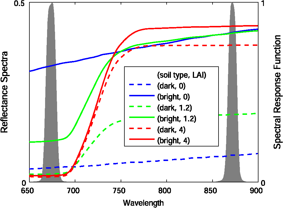

The input parameters for the canopy layer were obtained from the leaf chemical contents and the canopy biophysical and structural parameters. In this study, LAI was varied and all other parameters were held fixed, as summarized below. The leaf structure parameter was fixed at a value of 1.5, and the leaf properties were also fixed at levels of $40 μ g / {cm}^{2}$ chlorophyll, $8 μ g / {cm}^{2}$ carotenoid, 0.0 brown pigment, 0.01 cm leaf equivalent water, and $0.005 g / {cm}^{2}$ dry matter content. The canopy structural parameters assumed a spherical leaf angle distribution with a hot spot parameter of 0.01. The illumination and viewing conditions were assumed to be characterized by fixed values corresponding to a solar zenith angle (30 deg), a view zenith angle (10 deg), or a relative azimuthal angle (0 deg) over the entire simulation. Finally, the values of LAI were varied from 0 to 4 in intervals of 0.5.

The TOC reflectance spectra simulations obtained under the above conditions yielded a set of reflectance spectra (Fig. 5). These spectra were convoluted into band reflectances based on the band pass filters. The red and NIR bands were fixed using the band pass filters two and three, respectively, of the greenhouse gasses observing satellite cloud and aerosol imager (GOSAT-CAI). The CAI band two (red) ranged from 664 to 684 nm and band three (NIR) ranged from 860 to 880 nm, as shown in Fig. 5.

The soil line in the red–NIR reflectance space was then determined from the simulated band reflectances. The band reflectances were then simulated from the set of reflectance spectra, and the simulated band reflectances were tagged according to the value of LAI and the soil red reflectance $R_{s}$ . The slope $s_{1}$ and offset $s_{0}$ of the soil line were 1.2322 and 0.0260, respectively.

Finally, the parameters for the power series of $ρ_{n}^{'}$ were obtained from a polynomial fit after transforming the original red–NIR reflectance subspace based on the numerically simulated soil line. Figure 6 shows a plot of the soil isolines represented by an index-like parasite parameter $ρ_{n}^{'}$ [Eqs. (19) and (20)]. The results obtained using polynomials of three different orders (each band was modeled using a polynomial of order at most three) are compared in the figure. The simulated reflectance spectra (empty circles) are plotted in the figure to indicate the true soil isolines. As shown in the figure, the soil isolines agreed well with the simulated reflectance spectra when higher-order polynomials were used in the model ( $m_{p}$ ). Note that the distance between the soil isoline and the simulated reflectance spectrum is considered to be an error in the derived soil isoline equations. The figure shows that an order of three yields a very small error, indicating the high accuracy of the soil isoline equation. The next section discusses an investigation of the accuracy of the approximated soil isolines introduced in Sec. 4. The distance between a reflectance spectrum and an approximated soil isoline was calculated.

Fig. 6

Soil isolines represented by an index-like parasite parameter $ρ_{n}^{'}$ [Eqs. (19) and (20)]. The orders of the polynomials were one, two, or three for both bands. The simulated reflectance spectra are indicated by empty circles and provide references for the true spectra. The soil isolines derived in this study approached the true spectra (empty circle) as the order of polynomial increased.

5.2.

Accuracies of the Approximated Soil Isoline Equations

The accuracies of the approximated soil isoline equations described in Sec. 4 depended on the order of the polynomial used in Eqs. (29) and (30). The choice of the polynomial order in the two equations can differ, as in the asymmetric case described in the previous section. In this section, we assumed a polynomial order of at most three. Nine combinations of the integers $m_{r}$ and $m_{n}$ were possible, as summarized in Table 2. The table summarizes all nine combinations of the polynomial orders used in Eqs. (29) or (30) and the corresponding equations derived in Sec. 4. Figure 7 shows a plot of the approximated soil isolines obtained from six cases. The errors, measured based on the distance between the reflectance spectrum (empty circle) and the soil isolines, differed among the cases.

Table 2

References for each soil isoline equation, constructed using combinations of polynomial orders, mr and mn.

		$m_{n}$
		1	2	3
$m_{r}$	1	Eq. (34) in Sec. 4.1	Eq. (38) in Sec. 4.2	Eq. (38) in Sec. 4.2
	2	Eq. (40) in Sec. 4.3	Eq. (45) in Sec. 4.4	Eqs. (29) and (30) in Sec. 4
	3	Eq. (40) in Sec. 4.3	Eqs. (29) and (30) in Sec. 4	Eqs. (29) and (30) in Sec. 4

Fig. 7

Reflectance spectra and approximated soil isoline equations.

Figures 8(a) to 8(i) show the errors (on the logarithmic scale) obtained for the approximated soil isolines of the nine cases summarized in Table 2, as a function of $R_{s}$ and LAI. The error $ε (R_{s}, L)$ was computed as the distance between the simulated reflectance spectrum ( $ρ_{r}$ , $ρ_{n}$ ) and the reflectance spectrum on the soil isolines ( ${\hat{ρ}}_{r}$ , ${\hat{ρ}}_{n}$ ) for each pair of $R_{s}$ and LAI values.

Eq. (51)

ε (R_{s}, L) = \sqrt{{(ρ_{r} - {\hat{ρ}}_{r})}^{2} + {(ρ_{n} - {\hat{ρ}}_{n})}^{2}} .

Fig. 8

The error $\log_{10} ε (R_{s}, L)$ of the approximated soil isoline equations as a function of $R_{s}$ and LAI. The errors are defined as the distance between the approximated soil isolines and the simulated reflectance spectra.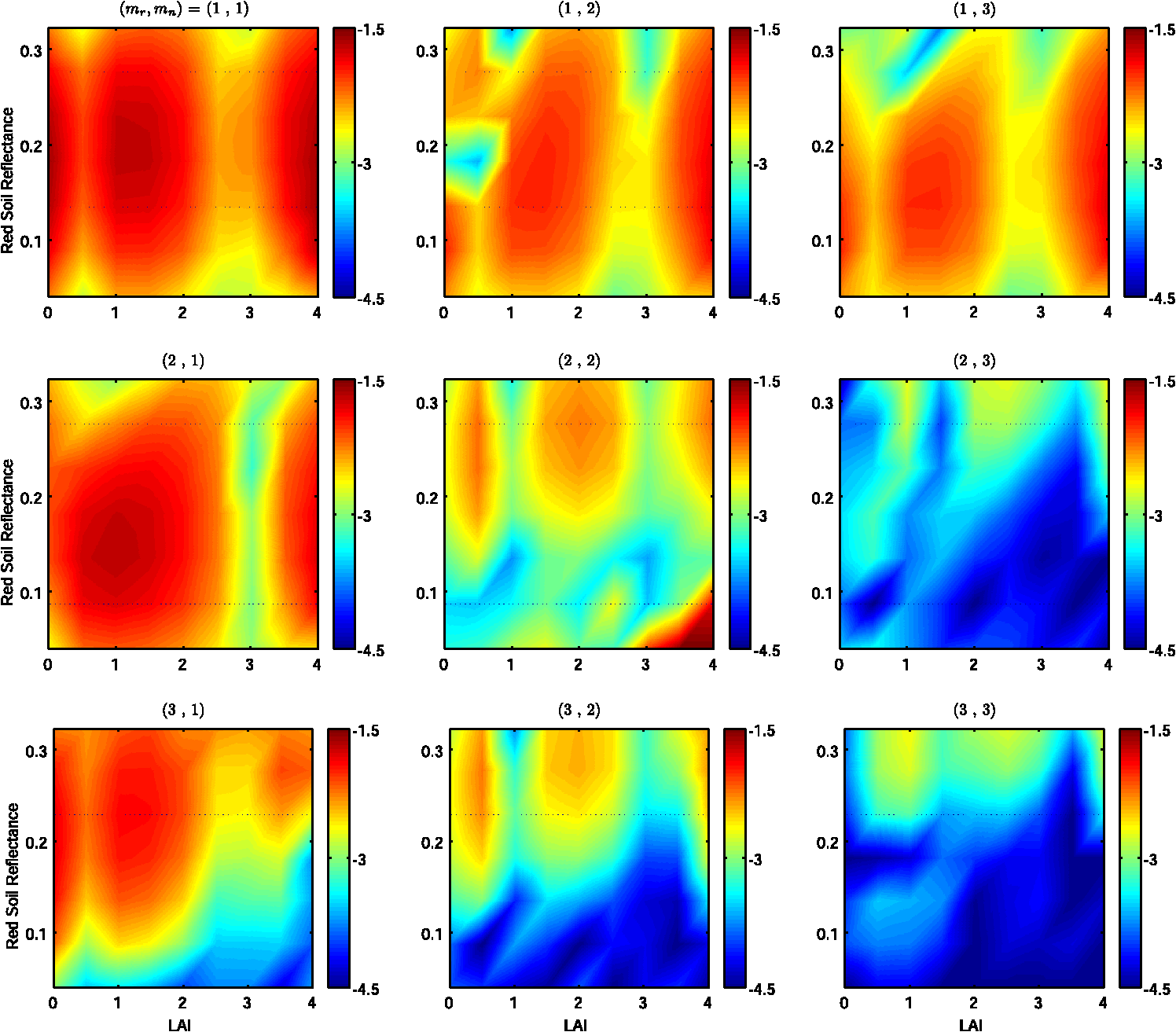

Models in which the truncation orders in the two bands were asymmetric yielded errors that were larger in the middle range of both $R_{s}$ and LAI parameter values. The overall error was low in the cases in which the NIR band was described using a higher-order polynomial, such as the cases of (1,2) and (1,3), unlike the reciprocal cases (2,1) and (3,1). The symmetric cases (1,1), (2,2), and (3,3) revealed that the error decreased as the polynomial order increased, as expected.

The trend in the errors of the soil isoline equations was characterized by averaging the error $ε (R_{s}, L)$ over the range of LAI values tested. Figure 9 shows the resulting errors as a function of only the soil red reflectance $R_{s}$ . The lower-order polynomial cases clearly displayed maximal errors in the middle of the range of $R_{s}$ values (0.2), whereas the use of a higher-order polynomial in either or both equations shifted the value of $R_{s}$ that produced the maximum error toward either higher or lower values of $R_{s}$ .

Fig. 9

Averaged error of the approximated soil isoline equations as a function of $R_{s}$ . The errors in Fig. 8 were averaged over the entire range of LAI.

Similarly, the error trend as a function of LAI was computed by averaging $ε (R_{s}, L)$ over the range of $R_{s}$ values. Figure 10 shows a trend distinct from that shown in Fig. 9. Interestingly, the local minima occurred at two LAI values ( $LAI = 0.5$ and 3) for most of the nine cases. In other words, the averaged error somehow increased in the middle range of LAI values ( $1 < LAI < 2$ ). This fact suggested that if one could improve the accuracy of the soil isoline in the middle range of LAI values, the overall error would improve dramatically, even in models based on lower-order polynomials. This possibility is worth investigating in future studies.

Fig. 10

Averaged error of the approximated soil isoline equations as a function of LAI. The errors in Fig. 8 were averaged over the entire range of $R_{s}$ .

Finally, the overall accuracy of the nine cases was evaluated by averaging over the entire range of values of $R_{s}$ and LAI (Table 3). Table 3 shows that the order of accuracy decreased as the polynomial order increased, whereas the asymmetric cases required special attention in the middle ranges of both LAI and $R_{s}$ parameters, as shown in Figs. 8, 9, and 10.

Table 3

Averaged errors of the soil isolines over the entire ranges of Rs and leaf area index values.

		$m_{n}$
		1	2	3
$m_{r}$	1	$9.6 \times 10^{- 3}$	$5.2 \times 10^{- 3}$	$4.7 \times 10^{- 3}$
	2	$7.4 \times 10^{- 3}$	$3.6 \times 10^{- 3}$	$0.43 \times 10^{- 3}$
	3	$4.5 \times 10^{- 3}$	$1.2 \times 10^{- 3}$	$0.37 \times 10^{- 3}$

6. Discussion

This study introduced a parametric form of the soil isoline equation in which an index was used as a parasitic parameter. Numerical difficulties associated with singularities in the original subspace were overcome by rotating the red and NIR axes through an angle equal to the soil line slope. Although the derived form included a parasitic parameter, a polynomial of arbitrary order may be used to represent the soil isoline equation. The derived parametric form suffered from the drawback that the soil isoline equation implicitly (rather than explicitly) described the relationship between the red and NIR reflectances.

An explicit form of the soil isoline was derived by considering a series of truncation cases. Although the relationships between the two reflectances were made explicit in these examples, the derived isoline equations presented truncation errors. Numerical investigations of the truncation errors in the derived forms clearly indicated that the error decreased as the truncation order increased.

The choice of truncation order may be asymmetric, such that the order of the polynomial describing the red band is not identical to that of the NIR band. An NIR band truncation order that exceeds that of the red band tends to yield smaller errors compared to the case in which the opposite holds. Photons at NIR wavelengths tend to scatter more frequently than photons with red wavelengths. This transport mechanism also suggests that higher-order terms should be used for the NIR bands to reduce truncation errors for cases in which the truncation orders of the two bands differ. The numerical results indicated that the overall accuracy of the approximated soil isoline equations decreased along with the truncation order, as expected. High truncation orders exceeding two reduced the error to $< 0.1 %$ .

In conclusion, the soil isoline equations derived here were reasonably accurate and enabled the use of expressions for further analysis of remotely sensed satellite data. Applications of the derived equations will be explored in future studies.

References

1.

A. R. Huete, “A soil-adjusted vegetation index (SAVI),” Remote Sens. Environ., 25 (3), 295 –309 (1988). http://dx.doi.org/10.1016/0034-4257(88)90106-X RSEEA7 0034-4257 Google Scholar

2.

F. BaretG. Guyot, “Potentials and limits of vegetation indices for LAI and APAR assessment,” Remote Sens. Environ., 35 (2), 161 –173 (1991). http://dx.doi.org/10.1016/0034-4257(91)90009-U RSEEA7 0034-4257 Google Scholar

3.

J. C. PriceW. C. Bausch, “Leaf area index estimation from visible and near-infrared reflectance data,” Remote Sens. Environ., 52 (1), 55 –65 (1995). http://dx.doi.org/10.1016/0034-4257(94)00111-Y RSEEA7 0034-4257 Google Scholar

4.

Z. LiX. Guo, “Leaf area index estimation in semiarid mixed grassland by considering both temporal and spatial variations,” J. App. Remote Sens., 7 (1), 073567 (2013). http://dx.doi.org/10.1117/1.JRS.7.073567 1931-3195 Google Scholar

5.

A. TongY. He, “Comparative analysis of SPOT, Landsat, MODIS, and AVHRR normalized difference vegetation index data on the estimation of leaf area index in a mixed grassland ecosystem,” J. App. Remote Sens., 7 (1), 073599 (2013). http://dx.doi.org/10.1117/1.JRS.7.073599 1931-3195 Google Scholar

6.

R. J. KauthG. S. Thomas, “The tasseled cap-a graphic description of the spetral-temporal development of agricultural crops as seen by Landsat,” in Symp. on Machine Processing of Remotely Sensed Data, 4B41 –4B51 (1976). Google Scholar

7.

C. J. Tucker, “Red and photographic infrared linear combinations for monitoring vegetation,” Remote Sens. Environ., 8 (2), 127 –150 (1979). http://dx.doi.org/10.1016/0034-4257(79)90013-0 RSEEA7 0034-4257 Google Scholar

8.

M. M. VerstraeteB. PintyR. B. Myneni, “Potentials and limitations of information extraction on the terrestrial biosphere from satellite remote sensing,” Remote Sens. Environ., 58 (2), 201 –214 (1996). http://dx.doi.org/10.1016/S0034-4257(96)00069-7 RSEEA7 0034-4257 Google Scholar

9.

M. M. VerstraeteB. Pinty, “Designing optimal spectral indexes for remote sensing applications,” IEEE Trans. Geosci. Remote Sens., 34 (5), 1254 –1265 (1996). http://dx.doi.org/10.1109/36.536541 IGRSD2 0196-2892 Google Scholar

10.

F. Liuet al., “Designing an improved soil moisture index in the near-infrared and shortwave plane,” in IEEE Int. Geoscience and Remote Sensing Symp., 3074 –3077 (2011). Google Scholar

11.

A. R. Huete, “Soil influences in remotely sensed vegetation-canopy spectra,” Theory and Application of Optical Remote Sensing, 107 –141 Wiley, New York (1989). Google Scholar

12.

C. F. Jordan, “Derivation of leaf area index from quality of light on the forest floor,” Ecology, 50 (4), 663 –666 (1969). http://dx.doi.org/10.2307/1936256 ECOLAR 0012-9658 Google Scholar

13.

J. W. Rouseet al., “Monitoring vegetation systems in the Great Plains with ERTS,” in 3rd ERTS Symp., 48 –62 (1973). Google Scholar

14.

J. G. P. W Clevers, “The derivation of a simplified reflectance model for the estimation of leaf area index,” Remote Sens. Environ., 25 (1), 53 –70 (1988). http://dx.doi.org/10.1016/0034-4257(88)90041-7 RSEEA7 0034-4257 Google Scholar

15.

A. J. RichardsonJ. H. Everitt, “Using spectral vegetation indices to estimate rangeland productivity,” Geocarto Int., 7 (1), 63 –69 (1992). http://dx.doi.org/10.1080/10106049209354353 1010-6049 Google Scholar

16.

A. R. Hueteet al., “Overview of the radiometric and biophysical performance of MODIS vegetation indices,” Remote Sens. Environ., 83 (1), 195 –213 (2002). http://dx.doi.org/10.1016/S0034-4257(02)00096-2 RSEEA7 0034-4257 Google Scholar

17.

Z. Jianget al., “Development of a two-band enhanced vegetation index without a blue band,” Remote Sens. Environ., 112 (10), 3833 –3845 (2008). http://dx.doi.org/10.1016/j.rse.2008.06.006 RSEEA7 0034-4257 Google Scholar

18.

J. Qiet al., “A modified soil adjusted vegetation index,” Remote Sens. Environ., 48 (2), 119 –126 (1994). http://dx.doi.org/10.1016/0034-4257(94)90134-1 RSEEA7 0034-4257 Google Scholar

19.

M. A. Gilabertet al., “A generalized soil-adjusted vegetation index,” Remote Sens. Environ., 82 (2), 303 –310 (2002). http://dx.doi.org/10.1016/S0034-4257(02)00048-2 RSEEA7 0034-4257 Google Scholar

20.

A. J. RichardsonC. L. Weigand, “Distinguishing vegetation from soil background information,” Photogramm. Eng. Remote Sens., 43 (12), 1541 –1552 (1977). PGMEA9 0099-1112 Google Scholar

21.

G. RondeauxM. StevenF. Baret, “Optimization of soil-adjusted vegetation index,” Remote Sens. Environ., 55 (2), 95 –107 (1996). http://dx.doi.org/10.1016/0034-4257(95)00186-7 RSEEA7 0034-4257 Google Scholar

22.

H. Yoshiokaet al., “Analysis of vegetation isolines in red-NIR reflectance space,” Remote Sens. Environ., 74 (2), 313 –326 (2000). http://dx.doi.org/10.1016/S0034-4257(00)00130-9 RSEEA7 0034-4257 Google Scholar

23.

H. Yoshioka, “Vegetation isoline equations for an atmosphere-canopy-soil system,” IEEE Trans. Geosci. Remote Sens., 42 (1), 166 –175 (2004). http://dx.doi.org/10.1109/TGRS.2003.817793 IGRSD2 0196-2892 Google Scholar

24.

F. BaretG. GuyotD. Major, “TSAVI: a vegetation index which minimizes soil brightness effects on LAI and APAR estimation,” in IEEE Int. Geoscience and Remote Sensing Symp., 1355 –1358 (1989). Google Scholar

25.

A. R. Huete, “Soil-dependent spectral response in a developing plant canopy,” Agron. J., 79 (1), 61 –68 (1987). http://dx.doi.org/10.2134/agronj1987.00021962007900010013x AGJOAT 0002-1962 Google Scholar

26.

H. YoshiokaA. R. HueteT. Miura, “Derivation of vegetation isoline equations in red-NIR reflectance space,” IEEE Trans. Geosci. Remote Sens., 38 (2), 838 –848 (2000). http://dx.doi.org/10.1109/36.842012 IGRSD2 0196-2892 Google Scholar

27.

F. BaretS. JacquemoudJ. F. Hancoq, “About the soil isoline concept in remote sensing,” Adv. Space Res., 13 (5), 281 –284 (1993). http://dx.doi.org/10.1016/0273-1177(93)90560-X ASRSDW 0273-1177 Google Scholar

28.

Z. Jianget al., “Interpretation of the modified soil-adjusted vegetation index isolines in red-NIR reflectrance space,” J. App. Remote Sens., 1 (1), 013503 (2007). http://dx.doi.org/10.1117/1.2709702 1931-3195 Google Scholar

29.

S. Jacquemoudet al., “Extraction of vegetation biophysical parameters by inversion of the PROSPECT+SAIL models on sugar beet canopy reflectance data. Application to TM and AVIRIS sensors,” Remote Sens. Environ., 52 (3), 163 –172 (1995). http://dx.doi.org/10.1016/0034-4257(95)00018-V RSEEA7 0034-4257 Google Scholar

30.

S. JacquemoudF. Baret, “PROSPECT: a model of leaf optical properties spectra,” Remote Sens. Environ., 34 (2), 75 –91 (1990). http://dx.doi.org/10.1016/0034-4257(90)90100-Z RSEEA7 0034-4257 Google Scholar

31.

S. Jacquemoudet al., “PROSPECT+SAIL models: a review of use for vegetation characterization,” Remote Sens. Environ., 113 (Suppl. 1), 556 –566 (2009). http://dx.doi.org/10.1016/j.rse.2008.01.026 RSEEA7 0034-4257 Google Scholar

32.

W. Verhoef, “Light scattering by leaf layers with application to canopy reflectance modeling: the SAIL model,” Remote Sens. Environ., 16 (2), 125 –141 (1984). http://dx.doi.org/10.1016/0034-4257(84)90057-9 RSEEA7 0034-4257 Google Scholar

33.

R. D. JacksonA. R. Huete, “Interpreting vegetation indices,” Prev. Vet. Med., 11 (3), 185 –200 (1991). http://dx.doi.org/10.1016/S0167-5877(05)80004-2 0167-5877 Google Scholar

34.

A. R. HueteR. D. Jackson, “Suitability of spectral indices for evaluating vegetation characteristics on arid rangelands,” Remote Sens. Environ., 23 (2), 213 –232 (1987). http://dx.doi.org/10.1016/0034-4257(87)90038-1 RSEEA7 0034-4257 Google Scholar

35.

A. R. HueteR. D. JacksonD. F. Post, “Spectral response of a plant canopy with different soil backgrounds,” Remote Sens. Environ., 17 (1), 37 –53 (1985). http://dx.doi.org/10.1016/0034-4257(85)90111-7 RSEEA7 0034-4257 Google Scholar

36.

H. Yoshiokaet al., “Derivation of soil line influence on two-band vegetation indices and vegetation isolines,” Remote Sens., 1 (4), 842 –857 (2009). http://dx.doi.org/10.3390/rs1040842 17LUAF 2072-4292 Google Scholar

37.

L. ShenY. HeX. Guo, “Suitability of the normalized difference vegetation index and the adjusted transformed soil-adjusted vegetation index for spatially characterizing loggerhead shrike habitats in North American mixed prairie,” J. App. Remote Sens., 7 (1), 073574 (2013). http://dx.doi.org/10.1117/1.JRS.7.073574 1931-3195 Google Scholar

38.

H. YoshiokaH. YamamotoT. Miura, “Use of an isoline-based inversion technique to retriave a leaf area index for inter-sensor calibration of spectral vegetation index,” in IEEE Int. Geoscience and Remote Sensing Symp., 1639 –1641 (2002). Google Scholar

39.

A. Kallelet al., “Determination of vegetation cover fraction by inversion of a four-parameter model based on isoline parameterizaion,” Remote Sens. Environ., 111 (4), 553 –566 (2007). http://dx.doi.org/10.1016/j.rse.2007.04.006 RSEEA7 0034-4257 Google Scholar

40.

H. YoshiokaA. R. HueteT. Miura, “An isoline-based translation technique of spectral vegetation index using EO-1 Hyperion data,” IEEE Trans. Geosci. Remote Sens., 41 (6), 1363 –1372 (2003). http://dx.doi.org/10.1109/TGRS.2003.813212 IGRSD2 0196-2892 Google Scholar

41.

K. ObataT. MiuraH. Yoshioka, “Derivation of a MODIS-compatible enhanced vegetation index from VIIRS spectral reflectances using vegetation isoline equations,” J. App. Remote Sens., 7 (1), 073467 (2013). http://dx.doi.org/10.1117/1.JRS.7.073467 1931-3195 Google Scholar

42.

H. YoshiokaT. MiuraK. Obata, “Derivation of relationships between spectral vegetation indices from multiple sensors based on vegetation isolines,” Remote Sens., 4 (3), 583 –597 (2012). http://dx.doi.org/10.3390/rs4030583 17LUAF 2072-4292 Google Scholar

43.

Y. Kimet al., “Spectral compatibility of vegetation indices across secsors: band decomposition analysis with Hyperion data,” J. App. Remote Sens., 4 (1), 043520 (2010). http://dx.doi.org/10.1117/1.3400635 1931-3195 Google Scholar

44.

A. P. TrishchenkoJ. CihlarZ. Li, “Effects of spectral response function on surface reflectance and NDVI measured with moderate resolution satellite sensors,” Remote Sens. Environ., 81 (1), 1 –18 (2002). http://dx.doi.org/10.1016/S0034-4257(01)00328-5 RSEEA7 0034-4257 Google Scholar

45.

N. V. Shabanovet al., “Analysis of interannual changes in northern vegetation activity observed in AVHRR data from 1981 to 1994,” IEEE Trans. Geosci. Remote Sens., 40 (1), 115 –130 (2002). http://dx.doi.org/10.1109/36.981354 IGRSD2 0196-2892 Google Scholar

46.

N. V. Shabanovet al., “Analysis and optimization of the MODIS leaf area index algorithm retrievals over broadleaf forests,” IEEE Trans. Geosci. Remote Sens., 43 (8), 1855 –1865 (2005). http://dx.doi.org/10.1109/TGRS.2005.852477 IGRSD2 0196-2892 Google Scholar

47.

K. Taniguchiet al., “Parametiric representation of soil isoline equation and its accuracy estimation in red-NIR reflectance space,” Proc. SPIE, 8524 85241J (2012). http://dx.doi.org/10.1117/12.977322 PSISDG 0277-786X Google Scholar

48.

H. YoshiokaK. Obata, “Soil isoline equation in red-NIR reflectance space for cross calibration of NDVI between sensors,” in IEEE Int. Geoscience and Remote Sensing Symp., 3082 –3085 (2011). Google Scholar

49.

K. Taniguchiet al., “Validity of soil isoline equation for a system of canopy and soil layers,” in IEEE Int. Geoscience and Remote Sensing Symp., 2613 –2616 (2013). Google Scholar

50.

C. AtzbergerK. Richter, “Spatially constrained inversion of radiative transfer models for improved LAI mapping from future Sentinel-2 imagery,” Remote Sens. Environ., 120 208 –218 (2012). http://dx.doi.org/10.1016/j.rse.2011.10.035 RSEEA7 0034-4257 Google Scholar

51.

C. Atzbergeret al., “Why confining to vegetation indices? Exploiting the potential of improved spectral observations using radiative transfer models,” Proc. SPIE, 8174 81740Q (2011). http://dx.doi.org/10.1117/12.898479 PSISDG 0277-786X Google Scholar

52.

C. AtzbergerK. Richter, “Geostatistical regularization of inverse models for the retieval of vegetation biophysical variables,” Proc. SPIE, 7478 74781O (2009). http://dx.doi.org/10.1117/12.830009 PSISDG 0277-786X Google Scholar

Biography

Kenta Taniguchi is an MS student at Aichi Prefectural University, Aichi, Japan. He received his BS degree in information science and technology from Aichi Prefectural University in 2012.

Kenta Obata is a postdoctoral fellow in the Institute of Geology and Geoinformation at the National Institute of Advanced Industrial Science and Technology, Japan. He received his MS and PhD degrees in information science and technology from Aichi Prefectural University, Aichi, Japan, in 2008 and 2010, respectively. His research interests include intersensor calibration of biophysical retrievals, spectral mixture analysis, and radiometric calibration.

Hiroki Yoshioka is a professor in the Department of Information Science and Technology at Aichi Prefectural University, Aichi, Japan. He received his MS and PhD degrees in nuclear engineering from the University of Arizona, Tucson, in 1993 and 1999, respectively. His research interests include cross-calibrations of satellite data products for continuity and compatibility of similar data sets, development of canopy radiative transfer models, and their inversion techniques.

CC BY: © The Authors. Published by SPIE under a Creative Commons Attribution 4.0 Unported License. Distribution or reproduction of this work in whole or in part requires full attribution of the original publication, including its DOI.

Citation Download Citation

Kenta Taniguchi, Kenta Obata, and Hiroki Yoshioka "Derivation and approximation of soil isoline equations in the red–near-infrared reflectance subspace," Journal of Applied Remote Sensing 8(1), 083621 (3 June 2014). https://doi.org/10.1117/1.JRS.8.083621

Published: 3 June 2014

Access the abstract

JOURNAL ARTICLE
19 PAGES

DOWNLOAD PAPER SAVE TO MY LIBRARY

GET CITATION

CITATIONS

Cited by 10 scholarly publications.

Explore citations on Lens.org

KEYWORDS

Reflectivity

Near infrared

Soil science

Vegetation

Data modeling

Computer simulations

Algorithm development

1.

Introduction

Fig. 1

2.

Difficulty in Modeling Soil Isolines Using Polynomial Fitting Approaches

Eq. (1)

Fig. 2

3.

Parametric Representation of the Soil Isoline Equation

3.1.

Assumptions and Transformation

Eq. (2)

Eq. (3)

Eq. (4)

Eq. (5)

Eq. (6)

Eq. (7)

Eq. (8)

Eq. (9)

Eq. (10)

Eq. (11)

3.2.

Polynomial Model in the New Reflectance Space

Eq. (12)

Eq. (13)

Fig. 3

Eq. (14)

Fig. 4

3.3.

Parametric Representation of a Soil Isoline

Eq. (15)

Eq. (16)

Eq. (17)

Eq. (18)

Eq. (19)

Eq. (20)

Eq. (21)

Eq. (22)

3.4.

Symbolic Form of the Soil Isoline Equation Without ρn′

Eq. (23)

Eq. (24)

Eq. (25)

Eq. (26)

Eq. (27)

Eq. (28)

4.

Approximations of the Soil Isoline Equation

Eq. (29)

Eq. (30)

4.1.

Case 1 (mr, mn) = (1,1): First-Order Approximation of the Soil Isoline Equation

Eq. (31)

Eq. (32)

Eq. (33)

Eq. (34)

4.2.

Case 2 (mr, mn) = (1, N): Asymmetric First-Order-in-Red Approximation

Eq. (35)

Eq. (36)

Eq. (37)

Eq. (38)

Eq. (39)

4.3.

Case 3 (mr, mn) = (N,1): Asymmetric First-Order-in-NIR Approximation

Eq. (40)

Eq. (41)

4.4.

Case 4 (mr, mn) = (2, 2): Second-Order Approximation

Eq. (42)

Eq. (43)

Eq. (44)

Table 1

Eq. (45)

4.5.

Case 5 (mr, mn) = (Nr, Nn): Higher-Order Approximation

Eq. (46)

Eq. (47)

Eq. (48)

Eq. (49)

Symbolic Form of the Soil Isoline Equation Without $ρ_{n}^{'}$

Case 1 (m_r, m_n) = (1,1): First-Order Approximation of the Soil Isoline Equation

Case 2 (m_r, m_n) = (1, N): Asymmetric First-Order-in-Red Approximation

Case 3 (m_r, m_n) = (N,1): Asymmetric First-Order-in-NIR Approximation

Case 4 (m_r, m_n) = (2, 2): Second-Order Approximation

Case 5 (m_r, m_n) = (N_r, N_n): Higher-Order Approximation