2.1.

Slope-Based Filter

Slope-based filtering of ALS data was proposed by Vosselman.²³ A slope filter is similar to a 3-D filtering mask cone (Fig. 1) defined by two parameters, $w$ and $s$. $w$ is the window size of the mask cone, and $s$ is the slope that defines the cone’s opening angle. The cone peak is moved to each testing point and is then used to check whether a neighboring point lies within or below the cone. If such a point is found, the testing point is recognized as a nonground point. Hence, this slope-based filter can be used to check any other points existing under the cone. If the check is positive, then the testing point is labeled as nonground; otherwise, the testing point is considered to be a ground point [see Fig. 1(b)].

Fig. 1

Diagram of the slope-based filter and the filtering algorithm: (a) the visualization of the slope-based filter; (b) the visualization of the filtering algorithm. It can be seen that there are no points under the cone if the cone is at ground level, but there are if the cone is located at a nonground point.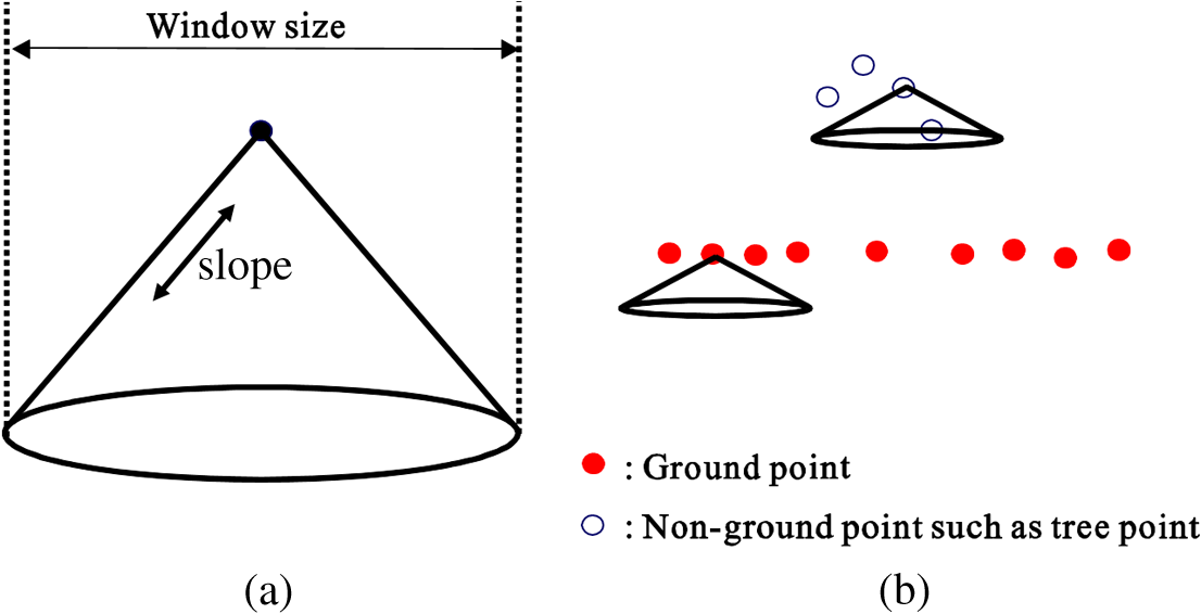

Terrain slope in the real world naturally varies in different locations; thus, using a fixed slope parameter is impractical. For this reason, Sithole¹⁹ proposed an AS filter that changes the slope threshold subject to the gradient over the local area covered by the filter. Preprocessing is usually needed to obtain an initial approximate ground surface in which the gradient can be estimated.

2.2.

Dual-Directional Slope-Based Filter

Although the AS filter has enough flexibility to deal with surfaces having various slopes, over-filtering problems in steep terrain areas still remain because this filter has a built-in assumption that the surface slopes do not vary rapidly. Figure 2 shows a schematic showing a possible over-filtering case for a terrain with very steep drop-offs. Under this circumstance, the interpolated DTM based on the resulting ground points will be over-smoothed because of the loss of some ground points near the most irregular areas [Fig. 2(c)]. To avoid over-filtering, we propose a DS filter, which is a modified version of the AS filter. The DS filter is a 1-D AS filter but is divided into two equal parts. Each part becomes a directional filter [Fig. 3(a)]. When applying these two directional filters to a profile, two sets of filtering results are obtained. Figure 3(b) shows a schematic illustrating the application of the DS filter to a cliff-like terrain. The union of the two resulting data sets is the final result of the DS filter [Fig. 3(c)]. The ground points near the cliff-like terrain are preserved.

Fig. 2

(a) A schematic over-filtering diagram of the application of the adaptive slope-based (AS) filter to a cliff-like terrain. (b) The reserved ground points. Note that some ground points near the cliff edges are removed. (c) The interpolated DTM with the reserved ground points is over-smoothed.

Fig. 3

A schematic diagram of filtering process using the dual-directional slope-based (DS) filter: (a) the DS filter is modified from the AS filter; (b) applying each DS filter to the profile points in Fig. 2(a), the filtered ground points using the two DS filters are obtained; (c) the final filtering result will be the union of the filtered points derived from each DS filter; note that the cliff topography is reserved.

2.3.

Filtering Algorithm of Dual-Directional Slope-Based Filter

The DS filter works along a 1-D space. To apply the DS filter, reorganization of point clouds must be prepared in advance. To this end, we segment point clouds into many strips in both the horizontal (east to west) and vertical (north to south) axes, as shown in Figs. 4(a) and 4(b). The point clouds are arranged into a grid. Each row and column of the grid is considered as a strip. The DS filter is then applied to each strip, which is also considered as a LiDAR profile. Filtering using the DS filter along either the horizontal or vertical axis should generally be sufficient because the cliff topography is kept either in the profile along the horizontal or vertical axis [e.g., Fig. 4(c-i)]. However, a special case will occur when the breaking line is parallel along either the vertical or horizontal axis [Figs. 4(c-ii) and 4(c-iii)]. In such cases, the DS filter can only demonstrate its advantage when it is applied to the profile in a direction perpendicular to the direction of the broken line. To avoid the possibility of ineffective filtering in such unusual cases, both the vertical and horizontal directions are selected in this study to segment point clouds. The width of each strip can be determined based on the density of the point clouds. The DS filter first works sequentially on the horizontal line and then repeats filtering on the vertical line [Figs. 4(a) and 4(b)].

Fig. 4

Point clouds are segmented into many strips in both the horizontal (a) and vertical directions (b) allowing the one-dimension DS filters to be applied to the strips for filtering purposes. The sub figure (c) makes clear that normally the cliff topography can be shown in the profile either along the horizontal axis or the vertical axis. (i) However, a special case will occur when the direction of the breaking line is along the vertical axis or (ii) the horizontal axis. (iii) In such two cases, only one profile will reveal the cliff topography.

At each strip, the DS filtering algorithm will result in two ground point data sets by the two DS filters with opposite directions. As a result, four sets of filtered points are obtained, that is two sets (${\text{Ground}}_1$, ${\text{Ground}}_2$) from the horizontal strips and two sets (${\text{Ground}}_3$, ${\text{Ground}}_4$) from the vertical strips. The final result ${\text{Ground}}_{\text{Final}}$ of the DS filtering algorithm is the union of the filtered ground point data sets, which is expressed as follows:

3.1.

Ground Seed Searching

The very low points, which are denoted as noise points, are first removed in this process. The noise points are typically relatively lower than the other near points. Noise points do not usually group together. These noise points can be classified using the conditions that the noise points have relatively low elevation and are isolated. We utilize the TerraScan module for the noise point classification. When the noise points are removed, a conventional slope-based filter²³ is applied to determine the best ground points to use as ground seeds. The conventional slope filter utilizes a fixed cone, with a shape controlled by a slope and its window size, which is applied to all point clouds. The slope must be set $<0.3$ based on our experiments to ensure that the searched points are ground points. The window size of the cone is the key parameter in this process, which must be set to a value larger than the longest side of objects (e.g., buildings). An urban area typically has large and dense buildings; thus, a wide window size should be set. However, a narrow window size is chosen to include numerous ground seeds. Based on our experiments and experiences, the window size is set at 20 to 70 m in cities and at 10 to 20 m in forest areas.

3.2.

Ground Region Growing and Dual-Directional Slope-Based Filtering

Once ground seeds are established, ground region growing can be conducted. This process refers to the determination of all possible ground points, in which some nonground points may be included. To implement this process, point clouds are segmented into numerous strips in both the horizontal and vertical directions in advance, as shown in Figs. 4(a) and 4(b). Thus, the neighboring relation between points can be established in each strip either in a horizontal or vertical direction. The region growing begins at each ground seed. If the elevation difference $\mathrm{\Delta }H$ between the seed point $p_o$ and its neighborhood $p_i$ is smaller than a threshold ($T$), then the neighborhood point ($p_i$) is labeled as a new seed. The process continues until the difference exceeds the threshold or meets another seed. The threshold $T$ is set according to the variations of the topographic relief. A large value of $T$ is used in steep terrains (3 m in our experiments); otherwise, $T$ is set not greater than 2 m. This process can generally remove obvious nonground points with elevations that are very high relative to the ground, that is, points representing such nonground elements as buildings or trees. All the selected ground seeds in this process may be considered as candidate ground points and will be further processed using the DS filters in the subsequent step. The candidate ground points are segmented into numerous LiDAR profiles, as mentioned in Sec. 2.3 and Fig. 4. The DS filtering algorithm is then applied to the generated profiles. Two parameters are needed for performing the DS algorithm. One parameter is the window size of the DS filter, which is set the same as the window size of the conventional filter used in ground seed searching (Sec. 3.1). The other parameter is the adaptive slope, which is derived based on the ground seeds covered by the window of the DS filter. After the DS filtering, the ground points are obtained.

4.1.

Test Data and Filters

The DS filter was compared with some known filters, including the filter indicated in the commercial software TerraSolid. Test data were downloaded from the ISPRS website ( http://www.itc.nl/isprswgIII-3/filtertest/index.html). Fifteen data sets extracted from a variety of terrains (S11 to S42 in urban areas with an average point density range of 1.0 to 1.5 m and S51 to S71 in rural areas with an average point density range of 2.0 to 3.5 m) were tested. Ground truth data (results of manual filtering) and the test results obtained using eight various methods are also provided on the website. We chose all eight filtering results for comparison to our algorithm. Among these methods, Axelsson’s algorithm yields better results than the others in most of the 15 data sets in terms of total error. A detailed description of the chosen filters and the test data set can be found in Sithole and Vosselman’s study.²¹ The classification accuracy of our algorithm was also compared with that of some recently proposed filtering algorithms.

We applied the AS filter and TerraSolid module (TerraScan) to the test data. The filtering principle of TerraScan utilizes Axelsson’s algorithm.²⁴ The advantages and shortcomings of the DS filter will be elucidated based on comparison to the results of the AS filter and TerraScan.

4.2.

Accuracy Assessment

Each point is classified as ground or nonground after filtering. A true positive (tp) occurs if a ground point is correctly classified as ground; a false negative (fn), which is also known as an omission error, occurs if a ground point is classified as nonground; a false positive (fp), which is also known as a commission error, occurs if a nonground point is classified as ground; a true negative (tn) occurs if a nonground point is correctly classified as a nonground. The commission errors usually cause a rough surface in the resulted DTMs and sometimes lead to a significant difference between the generated DTM and the real ground surface when a commission point’s elevation is higher than the ground. The omission error usually decreases the details of the ground surface, especially when the omission points represent a specific characteristic of the ground surface.

In this study, the classification results are judged in terms of type I error, type II error, total error, and Cohen’s kappa. All the assessment indices can be obtained using Eq. (2):

4.3.

Results and Analysis

The employed parameter values of the DS algorithm and the errors in each test site are shown in Table 1. The results indicate that the classification is generally better in urban areas (S11 to S42) than in rural areas (S51 to S71). This result could be due to the complexity of the surface features in the test area. Type I error, type II error, total error, and kappa values for the 15 samples processed using the eight methods in the report and our algorithm are compared in Tables 2 through 5, respectively. Based on the average of the four evaluation indices, the DS algorithm has the best performance in terms of type I error (3.42%), total error (4.32%), and kappa values (84.66%). Type II error is generally inverse to type I error for all the compared algorithms, of which the DS filtering algorithm has the worst result (9.28%). Such a result can be explained by the fact that filtering errors easily occur in the landscape boundary. The DS filter also needs geometric information in multidirections to judge a point, that is, either ground or nonground. When points locate near the landscape boundary, regions outside the test areas where no data were sensed will not provide the geometric information for the DS filtering algorithm to judge the points. Thus, filtering errors, either type I or II, could occur. Figures 6(d) and 6(h) show several example cases in which errors occurred near the boundaries when using the DS filter.

Table 1

The parameters and the classification accuracy of the dual-directional slope-based (DS) filter.

Table 2

Comparison of type I error for the 15 samples processed by using eight tested methods from the ISPRS report and DS filter.

Table 3

Comparison of type II error for the 15 samples processed by using eight tested methods from the ISPRS report and DS filter.

Table 4

Comparison of total error for the 15 samples processed by using eight tested methods from the ISPRS report and DS filter.

Table 5

Comparison of kappa values for the 15 samples processed by using eight tested methods from the ISPRS report and DS filter.

Fig. 6

(a) and (e) show the contour maps of site S52 and S53, respectively. (b)–(d) are filtering error distribution of site S52 using AS filter (b), Terrascan (c), and DS filter (d). (f)–(h) are filtering error distribution of site S53 using AS filter (f), Terrascan (g), and DS filter (d). The filtering errors in the circle indicate the limitation of DS filter that it easily results in filtering errors when the points are near the boundary of the test area.

For all the compared filters, type II error is generally low (under 10% for each of the 15 data sets). However, type I error results can reveal the filtering ability of the eight methods. Types I and II error results indicate that all the filters are capable of removing more commission errors than omission errors (considering that a low type II error necessarily means few commission errors, and all the filters have low type II error for the 15 data sets). The results also show that the total error correlates well with type I error rather than type II error. When all the filters have similar performances for type II error, type I error becomes the key factor in determining their final classification results, that is, their total error.

We also compared the total error and kappa values of the DS filtering algorithm with some other leading edge presented algorithms after 2009. The comparison result shown in Table 6 indicates that our algorithm is as good as the compared algorithms, except Pingel et al.’s algorithm, that achieved the lowest total error and the highest kappa value.

Table 6

Average total error and kappa values of six different filters and DS filter.

To further test the merit of the proposed DS filter with regard to handling ragged terrain, we applied and compared AS, TerraScan (using Axelsson’s algorithm), and the DS filter to study S52 and S53 which contain some ragged terrains. The spatial distributions of types I and II error for the three filters are shown in Fig. 6. The blue points in Fig. 6 indicate type I errors, which are mostly distributed on the ragged terrain. The results reveal that the AS algorithm has considerable type I errors [Figs. 6(b) and 6(f)]. Several of these type I errors are successfully avoided by the DS filter [Figs. 6(d) and 6(h)]. This result demonstrates the effectiveness of the modification from the AS filter to the DS filter by adding directional information. The TerraScan algorithm also performs better than the AS filter. However, the cliff in TerraScan algorithm’s results [Figs. 6(c) and 6(g)] erodes more than that in the DS algorithm’s results [Figs. 6(d) and 6(h)]. We also investigated the 3-D ground surfaces of S53 using the filtered ground points shown in Fig. 7. The ground surfaces were generated using the reference (a), AS-filtered (b), TerraScan-filtered (c), and DS-filtered ground points (d). The resulting ground surface generated using the DS algorithm can preserve sharp surfaces compared with that generated using AS and TerraScan algorithms. Therefore, the DS filter is more capable of keeping the ground points near the breaking lines rather than TerraScan and AS filters that tend to over-filter such ground points.

Fig. 7

Three-dimensional ground surface rendering of S53 by using the data from (a) reference ground points (considered as true ground surface), (b) AS ground points, (c) TerraScan ground points, and (d) DS ground points. The resulting ground surface generated using the DS algorithm can preserve sharp surface compared with that generated using AS and TerraScan algorithms (see the breaking lines inside the red polygon).