Improving image classification in a complex wetland ecosystem through image fusion techniques

Lalit Kumar; Priyakant Sinha; Subhashni Taylor

doi:10.1117/1.JRS.8.083616

11 June 2014 Improving image classification in a complex wetland ecosystem through image fusion techniques

Lalit Kumar, Priyakant Sinha, Subhashni Taylor

Author Affiliations +

Journal of Applied Remote Sensing, Vol. 8, Issue 1, 083616 (June 2014). https://doi.org/10.1117/1.JRS.8.083616

Abstract

The aim of this study was to evaluate the impact of image fusion techniques on vegetation classification accuracies in a complex wetland system. Fusion of panchromatic (PAN) and multispectral (MS) Quickbird satellite imagery was undertaken using four image fusion techniques: Brovey, hue-saturation-value (HSV), principal components (PC), and Gram–Schmidt (GS) spectral sharpening. These four fusion techniques were compared in terms of their mapping accuracy to a normal MS image using maximum-likelihood classification (MLC) and support vector machine (SVM) methods. Gram–Schmidt fusion technique yielded the highest overall accuracy and kappa value with both MLC (67.5% and 0.63, respectively) and SVM methods (73.3% and 0.68, respectively). This compared favorably with the accuracies achieved using the MS image. Overall, improvements of 4.1%, 3.6%, 5.8%, 5.4%, and 7.2% in overall accuracies were obtained in case of SVM over MLC for Brovey, HSV, GS, PC, and MS images, respectively. Visual and statistical analyses of the fused images showed that the Gram–Schmidt spectral sharpening technique preserved spectral quality much better than the principal component, Brovey, and HSV fused images. Other factors, such as the growth stage of species and the presence of extensive background water in many parts of the study area, had an impact on classification accuracies.

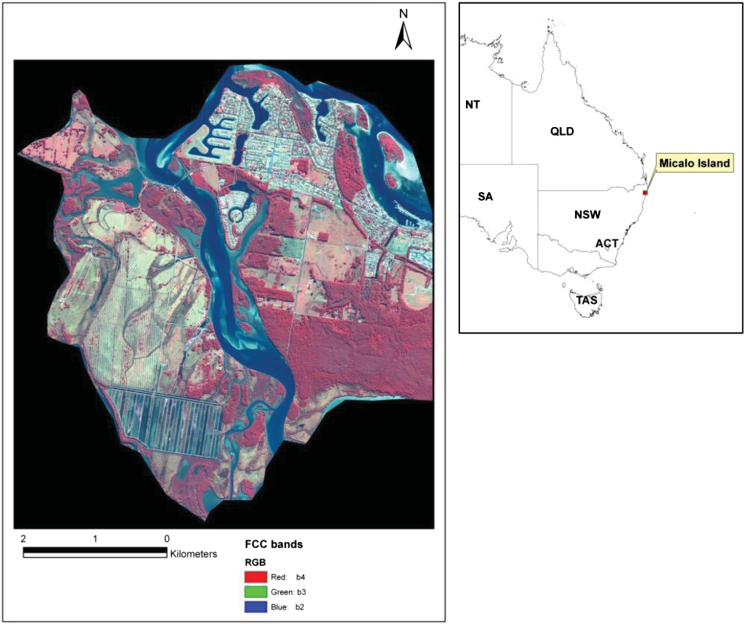
1. Introduction

Wetlands cover about 9% of the surface of the Earth and contain around 35% of global terrestrial carbon. They are good sinks for carbon dioxide and other greenhouse gases, especially if their vegetation is protected and their natural processes are maintained. Wetlands help to improve water quality by filtering pollutants, trapping sediments, and absorbing nutrients that would otherwise result in poor water quality downstream. They also provide habitats for wildlife as well as many valuable ecosystem services.¹ Coastal wetlands, such as saltmarsh and mangroves, are likely to have the highest rates of greenhouse gas sequestration, and the drainage of melaleuca and mangrove forest wetlands in Australia would turn them from carbon sinks into carbon sources.² Saltmarsh can bury an average of 1.51 tons of organic carbon per hectare per year.²^,³ This rate is several times higher than the rate of carbon sink calculated for the Amazonian forests, an important global carbon sink, and highlights the importance of protecting wetlands to mitigate the impacts of climate change. Coastal saltmarshes are also ecologically important habitats that link the marine and terrestrial environments and provide habitat for both marine and terrestrial organisms. They also provide an important buffer between land and reef, as they filter land runoff and improve the quality of water.⁴^,⁵

Saltmarshes have been subject to extensive exploitation, modiﬁcation, and destruction due to the effects of human activity.⁶ A significant proportion of the Australian eastern coast has been developed since European settlement. However, due to a lack of historical data, the actual area of mangrove and saltmarsh habitat loss is unknown. Continued research and monitoring are required to provide up-to-date information on mangrove and saltmarsh habitat boundaries, and to improve our ability to detect subtle changes in the condition of these communities. Mapping and modeling in saltmarshes face distinct challenges due to tidal oscillation and variability, fieldwork logistics, and the inherent dynamic nature of these environments.⁷

Remote sensing has been applied with increasing success in the monitoring and management of aquatic ecosystems.⁸^–¹² The occurrence of wetlands in diverse geographic areas makes it challenging to map such ecosystems.¹³ Improvements in sensor technology, particularly in terms of enhanced spectral and spatial resolutions, have made remote sensing a useful tool for mapping, monitoring, and assessing wetland environments.¹⁴^–¹⁸ Spatial resolution defines the degree of fine detail that can be seen in an image, while spectral resolution can be thought of as the width of the bandpass, in which the incoming radiance field is measured by the sensor.¹⁹ Multispectral (MS) remote sensing systems collect reflected energy from an object or area of interest in multiple bands (regions) of the electromagnetic spectrum, while panchromatic (PAN) systems collect reflected energy in one band.²⁰ For recording a similar amount of incoming energy, the spatial resolution of a PAN detector can be smaller than that of an MS detector. Thus, most sensors of earth resource satellites, such as SPOT, IKONOS, and Quickbird, provide PAN and MS images at different spatial resolutions.²¹ While the PAN image provides greater spatial resolution, the MS image provides greater spectral resolution, hence each image type has certain advantages over the other. Enhanced image or data fusion provides us with the opportunity to utilize the advantages of each of the images more effectively, particularly in change analysis.²²

Image fusion is the combination of two or more different images to form a new image by using various algorithms.²³^,²⁴ Pan sharpening is an example of image fusion, which involves merging high-spectral-resolution MS and high-spatial-resolution PAN images.²⁵ More specifically, a pan-sharpened MS image is a fusion product, in which the MS bands are sharpened through the higher-resolution PAN image. Image fusion can provide certain advantages in the mapping and monitoring of wetlands because the different types of vegetation or classes may be better classified if high-spatial- and spectral-resolution images are used. Improvements in the classification accuracy of remotely sensed images are achievable through the selection of suitable band combinations²⁶ and also through image enhancement, such as image fusion,²³ because higher-spatial-resolution data are used to select training sites, interpret classification results, and describe the spatial distribution and patterns of land cover.²⁷^,²⁸ However, the classification accuracy of fused imagery may depend on its spectral quality, which is largely determined by the fusion algorithm that is utilized. A number of studies have explored the impacts of different fusion algorithms on classification accuracies and have observed improvements,²⁹^–³² while others found that the classification accuracy of fused imagery was lower than the original MS image.³³

This study investigated the usefulness of image fusion techniques in wetland vegetation mapping to ascertain whether image fusion improved the classification accuracy in a complex wetland ecosystem. The impact of four fusion techniques, Brovey, hue-saturation-value (HSV), principal components (PC) spectral sharpening, and Gram–Schmidt (GS) spectral sharpening, on the classification accuracy for wetland vegetation mapping was examined using two classification methods.

2. Materials and Methods

2.1.

Study Site

The study was carried out at Micalo, situated on the eastern coast of New South Wales, Australia, between 153° 17′ 50′′ E to 153° 21′ 03′′ E longitude and 29° 24′ 45′′ S to 29° 28′ 25′′ S latitude (Fig. 1). It covers approximately 950 ha and includes both terrestrial and estuarine habitats. The main saltmarsh vegetation species at Micalo are salt couch (Sporobolus virginicus), samphire (Sarcocornia quinqueflora), creeping brookweed (Samolus repens), Austral seablite (Sueda australis), and sea rush (Juncus krausii). The main nonsaltmarsh vegetation species are casuarina (Casuarina glauca), paperbark (Melaleuca quinquenervia), mangroves (Avicennia marina and Aegicerus corniculatum), pasture grass, tall reedy grass, and a number of shrub-type weeds. The vegetation species at the study site were fairly diverse, with a number of species in different stages of growth and maturity. Stands of S. quinqueflora in two different colors, reddish and very green, were found to occur short distances apart. Similar phase differences were also observed for S. virginicus: some were lush and green while others were tall and dry (Fig. 2). The study site, while located close to the coast, is not significantly impacted by coastal tides; however, there was a substantial amount of water in many parts. Permanent standing water constituted between 30% and 80% of the background in many areas, and this complicated vegetation categorization and image processing. Figure 2 shows the examples of diverse vegetation and the extent of water present in the background.

Fig. 1

Location of Micalo on the northeast coast of New South Wales, Australia. Image is a false-color Quickbird of July 12, 2004.

Fig. 2

Vegetation species at different stages of growth (a–d) and extent of background water (e, f) at the study site.

2.2.

Methods

High-spatial-resolution data from Quickbird were used in this study. Quickbird images have a 0.61-m pixel resolution in the PAN mode and 2.44-m resolution in the MS mode. The MS mode consists of four broadbands in the blue (450–520 nm), green (520–600 nm), red (630–690 nm), and near-infrared (760–900 nm). The Quickbird satellite data were captured on July 12, 2004.

Extensive fieldwork was conducted in the study area on the 20th and 21st of July, 2004. Data were collected for a total of 224 locations. Each of the sample sites was homogeneous area of at least $10 \times 10 m$ , so that the georeferencing issues would not have an impact on training sites. Ground data included main vegetation species, percentage occurrence of each species within the selected plots, crown cover and density, condition of the wetland, and their GPS locations. During the fieldwork, 33 ground control points were also collected using a differential GPS system for image rectification.

Image fusion was carried out using Quickbird MS and PAN imageries with different spectral and spatial resolutions to produce an image with enhanced spatial resolution. The four image fusion algorithms employed were Brovey, HSV, PC spectral sharpening, and GS spectral sharpening. Since the Brovey and HSV techniques only allow a limited number of input bands to be fused, bands containing most of the variance were selected based on the optimum index factor, a method developed by Chavez et al.³⁴

2.2.1.

Brovey transformation

A mathematical combination of the color image and high-spatial-resolution data is utilized in this sharpening technique, whereby each band in the color image is multiplied by a ratio of the high-spatial-resolution data divided by the sum of the color bands. A nearest neighbor technique is then used to resample each of the three color bands to the high-spatial-resolution pixel size.²⁵^,³⁵ The method is computationally simple and is generally the fastest method that requires the least system resources. The intensity component is increased, making this technique good for highlighting brighter objects. The method was developed to visually increase contrast in the low and high ends of an image histogram (i.e., to provide contrast in shadows, water, and high reflectance areas, such as urban features). However, the resulting merged image does not retain the radiometry of the input multispectral image.³¹ Furthermore, this technique allows only three bands at a time to be merged from the input multispectral image.³⁵

2.2.2.

HSV

This technique is also called IHS and involves a color space transformation. In such a transformation, an RGB image is converted into color (hue), purity (saturation), and intensity or brightness (value). The next step in this fusion algorithm involves replacing the value band with the high-spatial-resolution PAN band. The hue and saturation bands are then resampled to the high-spatial-resolution pixel size using a nearest neighbor technique. Histogram matching of the PAN image is carried out before substitution, which involves radiometrically transforming the PAN image by a constant gain and bias in such a way that it exhibits mean and variance that are the same as the intensity.³⁶ A final transformation of the image back to RGB color space is carried out.³⁵ Only three of the four bands at a time are merged from the input MS image because the HSV transform is defined for only three components. The HSV offers a controlled visual presentation of the data using readily identifiable and quantifiable color attributes that are distinctly perceived.³⁷ Numerical variations can be uniformly represented in an easily perceived range of colors. However, in HSV, the hue has to be carefully controlled since it associates meaningful color with well-defined characteristics of the input.³⁷

2.2.3.

PC

This method is based on the assumption that the first principal component of high variance is ideal for replacement with the high spatial details from the PAN image. The MS data are transformed using a principal components transformation. The high-spatial-resolution PAN is scaled to match the PC band 1 (PC1) to avoid distortion of the spectral information. This step is essential since the mean and variance of PC1 are generally far greater than those of the PAN. The PC1 band is then replaced with the scaled PAN. Finally, an inverse transformation is performed and the MS data are resampled to the high-spatial-resolution pixel using the nearest neighbor technique.³⁵ The PCA is mainly used to reduce dimensionality of the data while retaining useful information and also for image enhancement. The dimensionality reduction is desired to reduce data redundancy and processing time in color compositing.³⁸ It also has no limitation on the number of bands that can be merged at a time. However, with PCA, there is a possibility of losing important information if an unused image contains more signiﬁcant information than used images and there is difﬁculty in visual interpretation of color composition images due to fewer numbers of bands.³⁹ Information in spectral bands would not be preserved after implementing PCA, and merged low-resolution MS images are not easy to identify.³⁸

2.2.4.

GS

The lower spatial resolution spectral bands are used to simulate a PAN band. This step is followed by a GS transformation on the simulated band and the spectral bands, using the simulated PAN band as the first band. The high-spatial-resolution PAN band is substituted with the first GS band. The final step involves an inverse GS transform to generate the pan-sharpened spectral bands.³⁵ GS is typically more accurate because it uses the spectral response function of a given sensor to estimate what the PAN data look like. Karathanassi et al.⁴⁰ found local mean and variance matching, and least-squares fusion methods, the best performance in GS as compared to other methods; however, they also found that there was not a good comparison in the correlation coefficient value between the two images.

2.3.

Image Classification

2.3.1.

Maximum-likelihood classification

Saltmarsh landcover classification was carried out on the original Quickbird image bands (B1-4) and on the entire bands of the fused images. Maximum-likelihood classification (MLC) was used for image classification through (1) identification of features and selection of training areas based on field data, (2) evaluation and analysis of training signature statistics and spectral patterns, and (3) classification of the images. MLC works on two assumptions: (1) that the image data are normally distributed, and (2) that the training samples’ statistical parameters (e.g., mean vector and covariance matrix) truly represent the corresponding landcover class. However, the image derived parameters are not always normally distributed, especially in complex landscapes. Differential GPS-based reference samples collected during the field visit of the sites were first superimposed on standard false-color composites using 4 3 2 band combination and checked for class homogeneity around the sample points. Given the diverse nature of the vegetation and the large differences in the amount of water in the background, the landcover types were initially categorized into 20 groups. A key issue in deciding on landcover classes was how to handle the issue of background water. It was decided that where a particular vegetation species covered more than 80% of the sample area, it would be placed in the “pure” category, such as “S. quinqueflora pure”; where there was a mix of the vegetation and water, with water accounting for more than 20% but less than 50% of the area, the class was listed as the vegetation species being dominant, such as “S. quinqueflora dominant”; and where there was an even mix of vegetation species and water this class was listed as a mixed class.

A total of 224 sample points were collected for the 20 saltmarsh landcover classes, which were later grouped into nine classes by merging nearby classes into one, as there was a significant crossover between some classes due to high water cover. These sample points were used to make sample polygons of $3 \times 3 pixels$ . Given the fact that the positional accuracy of locations extracted from high-resolution images can be degraded by off-nadir acquisition and image distortion,⁴¹ the $3 \times 3 pixels$ accounted for any existing positional error. To avoid any class mixing, the $3 \times 3$ sample pixels were further refined with respect to class homogeneity by retaining only pure pixels in a given polygon and discarding pixels falling on class boundaries or neighboring class (Fig. 3). After refinement, a total of 1189 sample pixels were left for training and accuracy assessment processes. From the total sample pixels, 416 training pixels were randomly selected for signature generation and image classification, while the remaining samples were used for classification accuracy evaluations. Table 1 shows the number of samples per class used for training and accuracy assessment processes. Signatures were further refined using Jeffries–Matusita (JM) distance and transformed divergence (TD)³⁴ separability measures. Class homogeneity around the sample points was examined, and if required, a point was slightly moved to the adjacent pixel to accommodate more similar pixels in the surroundings. Finally, both the original and the fused images (resulting from various fusion techniques) were classified into nine saltmarsh landcover categories.

Fig. 3

Refinement of sample pixels by retaining only pure pixels in a given polygon by discarding pixels falling on class boundaries or neighboring class.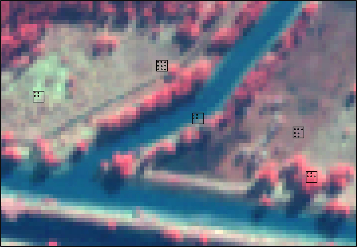

Table 1

Class-wise sample points used for training and accuracy assessment for saltmarsh landcover classifications in the study region.

Sample	Class	Training points	Accuracy assessment points
1	Casuarina + Mangrove + Melaleuca (CMM)	88	148
2	Grass	54	68
3	J. krausii + S. virginus dominant + S. virginus pure	98	196
4	Others (mixed S. repens, S. australis, and weeds, etc.)	13	14
5	Pasture	30	60
6	S. quinqueflora dominant	22	42
7	S. quinqueflora pure	30	59
8	Water	32	103
9	Settlements	49	83

2.3.2.

Support vector machines classification

SVM is a supervised classification method derived from statistical learning theory⁴² and found suitable for complex and noisy data classification. It separates the classes with a decision surface, often called the optimal hyperplane, which maximizes the margin between the classes. The data points closest to the hyperplane are called support vectors, critical elements of the training set. As a consequence, they generalize well and often outperform other algorithms in terms of classification accuracies. In addition, the misclassification error is minimized by maximizing the margin between the data points and the decision boundary. While SVM is a binary classifier in its simplest form involving separation of only two classes, it can function as a multiclass classifier by combining several binary SVM classifiers (creating a binary classifier for each possible pair of classes). The SVM-based classification involves separating data into training and testing sets. Each instance in the training set contains one “target value” (i.e., the class labels) and several “attributes” (i.e., the features or observed variables). The goal of SVM is to produce a model (based on the training data), which predicts the target values of the test data given only the test data attributes.

Given a training set as $(x_{i}, y_{i})$ , $i = 1, \dots l$ ; where $x_{i} \in R^{n}$ and $y_{i} \in {1, - 1}^{1}$ , the training set can be separated linearly by a hyperplane, if a vector $w$ and a scalar $b$ satisfy two conditions: $w * x_{i} + b \geq + 1$ for all $y = + 1$ ; and $w * x_{i} + b \leq + 1$ for all $y = - 1$ . The two conditions can be combined as $y_{i} (w * x_{i} + b) - 1 \geq 0$ to represent a constraint that must be satisfied to achieve a hyperplane that completely separates the two classes.⁴³ The SVM finds the optimal separating hyperplane using Lagrange multiplier and quadratic programming methods.⁴⁴ For cases where the two classes are not linearly separable, a mapping function “ $Φ$ ” is used as $Φ (x)$ , which is the conversion of input vector $x$ in feature space into a constructed space of $n$ dimensions. With increasing $n$ , this is computationally expensive and hence a kernel function, $K (x, y) = Φ (x) * Φ (y)$ , is chosen. The most commonly used kernels to build SVM for classification are the radial-based function (RBF) and polynomial-based function. The choice of kernel used and the parameters selected can have an effect on speed and accuracy of classification.⁴⁵ In principal, SVMs can only solve binary classification problems. One commonly used technique that allows for multiclass classification is the one-against-one method. This method fits a total of $k (k - 1) / 2$ binary subclassifiers and finds the correct class by a voting mechanism. The one-against-all method is an alternative approach, in which $k$ SVM models are constructed.⁴⁶ The $i$ ’th SVM is trained with all members of $i$ having positive labels, and all remaining members having negative labels.

In this study, the one-against-one method was used, as it has been shown that it performs better than the one-against-all method.⁴⁷ ENVI (ITT Visual Information Solution, US) was used for SVM classification based on the pairwise classification strategy for multiclass classification. SVM classification output is the decision value of each pixel for each class, which is used for probability estimates. The probability values were stored in ENVI as rule images, representing “true” probability in the sense that each probability falls in the range of 0–1, and the sum of these values for each pixel equals 1. The classification was performed by selecting the highest probability using the RBF kernel with $γ = 0.2$ as the inverse of the number of bands in the input image with a penalty parameter of 100 (default). The penalty parameter permits a certain degree of misclassification, which is particularly important for nonseparable training sets. Finally, a pixel-based SVM classification was undertaken by separating classes based on optimally defined hyperplane between class boundaries. Identical sets of training and validation samples were used for MLC and SVM classifications for all the fused images and also for the MS image to minimize evaluation bias.

2.4.

Accuracy Assessment

Accuracy of classifications was carried out to verify the fitness of classification products and to compare the performances of different image fusion techniques. The remaining 773 sample points were used for classification accuracy assessment bearing in mind the general guidelines for the minimum number of samples required for each landcover category.⁴¹ The evaluation was undertaken by comparing the location and class of each ground-truthed pixel with the corresponding location and class on the classified images. An error matrix was constructed expressing the accuracies in terms of producer’s accuracy (PA), user’s accuracy (UA), and overall accuracy (OA).⁴¹^,⁴⁸ This provided a means of expressing the accuracies of each individual class and their contribution to overall accuracy. Kappa coefficient ( $κ$ )⁴⁹^,⁵⁰ was also used to quantify how much better a particular classification was compared to a random classification and to calculate a confidence interval to statistically compare two or more classifications. One of the most widely used methods to compare accuracies is through the comparison of two independent kappa values. The statistical significance of the difference between the two values can be evaluated through the calculation of a $Z$ value.⁴¹ However, there are many issues related to the reliability of the interpretation of the kappa.⁵⁰ Therefore, it is preferable to express accuracies as the proportion of correctly allocated pixels (i.e., overall accuracy), as explained in Foody.⁵⁰ In this study, the same set of reference samples was used for all the classifications. Therefore, each set of reference samples can be treated as dependent samples for all the techniques that were applied. In such a situation, the significance of the difference between the two proportions (overall accuracy) has been evaluated using McNemar’s test⁵¹

Z = \frac{f_{12} - f_{21}}{\sqrt{f_{12} + f_{21}}},

where

f_{i j}

is the frequency of the validation data at row

i

, column

j

;

f_{12}

and

f_{21}

are the number of pixels that one method correctly classified as compared to the number of pixels the other method incorrectly classified.⁵¹ The test bases its evaluation on the

χ^{2}

distribution, in which the square of

Z

follows a

χ^{2}

distribution with one degree of freedom⁵⁰^,⁵¹ as

χ^{2} = \frac{{(f_{12} - f_{21})}^{2}}{f_{12} + f_{21}} .

3. Results

3.1.

Maximum-Likelihood-Based Classification Results

The main plant species that dominated the Micalo saltmarsh of the eastern coast of Australia were S. quinqueflora and S. virginicus. Saltmarsh landcover classifications from MLC technique produced different accuracies from the original MS image and the four fused images. An overall classification accuracy of 59% and kappa value of 0.55 were obtained from the original MS image involving all spectral bands. In general, the main confusion was observed between pure S. quinqueflora and dominant S. quinqueflora classes along with mixed wet vegetation types. Another class that could not be separated well was the category “others” of mixed vegetation types and was found to be similar in spectral response to J. krausii-dominated vegetation type. Table 2 summarizes the UA, PA, OA, and kappa values obtained for the nine landcover classes from different images used in MLC classification. With 13 and 16 different band combinations used in Brovey and HSV image fusion techniques, respectively, the classification accuracies from fused images with no infrared bands (e.g., RGB: 123) produced lower accuracies as compared to images with infrared bands (e.g., RGB: 432). For the Brovey method, the highest overall accuracies were 54% (kappa value 0.47) for noninfrared band images and 57.6% (kappa value 0.52) for images containing infrared as one of the bands in image fusion. With the same combinations in HSV technique, these values were 46.3% (kappa value 0.37) and 61.5% (kappa value 0.55), respectively. A similar pattern of class intermixing was observed between the fused images that yielded the highest accuracies and the classified original MS image. Nevertheless, the fused images showed an improvement of approximately 2% in overall accuracy and of 0.01 in kappa value over the original MS image. The Brovey technique resulted in a reduction in overall accuracy and kappa value by about 3% and 0.03, respectively, compared to the original MS image. Thus, this fusion technique does not look promising in terms of improving the classification accuracies in saltmarsh landcover classification.

Table 2

Comparison of landcover classification accuracies using different images from maximum-likelihood classification (MLC).

Class	Brovey (432)		HSV (432)		GS		PC		MS
Class	PA	UA	PA	UA	PA	UA	PA	UA	PA	UA
Casuarina+Mangrove+Melaleuca (CMM)	76.1	75.2	79.0	85.2	87.4	89.6	86.3	78.7	86.3	74.8
Grass	52.7	54.7	71.0	64.8	50.0	60.7	68.7	57.0	57.6	56.3
J. krausii + S. virginicus dominant + S. virginicus pure	20.4	67.2	30.0	67.5	38.8	73.0	17.6	58.0	22.0	74.5
Others (mixed S. repens, S. australis, weeds, etc.)	13.6	2.2	6.7	1.5	21.4	4.1	6.7	1.8	13.6	2.3
Pasture	84.2	61.2	90.2	63.8	91.7	83.3	87.0	83.5	75.4	69.1
S. quinqueflora dominant	25.0	15.8	27.5	23.9	19.0	18.6	45.0	39.1	27.5	18.1
S. quinqueflora pure	53.5	36.4	73.3	36.6	67.8	42.5	70.0	29.8	54.0	35.7
Water	99.6	100.0	83.8	100.0	100.0	100.0	89.9	100.0	100.0	100.0
Settlements	88.2	84.6	100.0	81.1	92.7	92.7	91.3	80.7	87.8	84.9
Overall accuracy	57.6		61.5		67.5		61.0		59.1
Kappa value	0.52		0.56		0.63		0.56		0.55

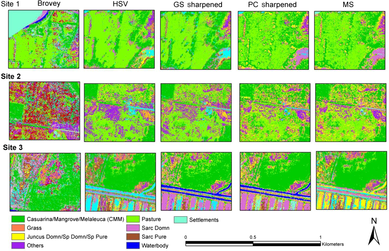
The landcover classification results from GS sharpened images were the best among all the MLC classifications, as it produced the highest overall accuracy of 67.5% and kappa value of 0.63, an improvement of approximately 8.5% in overall accuracy and 0.08 in kappa value, as compared to the original MS image classification. Confusion between classes such as pure S. quinqueflora, dominant S. quinqueflora, mixed wet vegetation, and “others” of mixed vegetation types was reduced, leading to higher producer and overall accuracies. For PC sharpened image, the overall accuracy was 61% (kappa value 0.56), an improvement of about 2% in overall accuracy and of 0.01 in kappa value over the original image classification. Overall, water and settlement were classified accurately by all the fused images, while among the vegetation types, CMM, grass, and pastures were separable in most cases. Figure 4 shows three areas in the study site comparing the classification results of the MS and four fused images.

Fig. 4

Three sample sites in the study area where the classification results vary between the multispectral (MS) and different fused images using maximum-likelihood classification (MLC) method.

3.2.

Support Vector Machines–Based Classification Results

The SVM method resulted in higher accuracies for all the image types compared to the MLC method. Table 3 summarizes the UA, PA, OA, and kappa values obtained for the nine landcover classes from different images used in SVM classification. Overall, the improvements of 4.1%, 3.6%, 5.8%, 5.4%, and 7.2% in overall accuracies were obtained in case of SVM over MLC for Brovey, HSV, GS, PC, and MS images, respectively.

Table 3

Comparison of landcover classification accuracies using different images from a support vector machine (SVM).

Class	Brovey (432)		HSV (432)		GS		PC		MS
Class	PA	UA	PA	UA	PA	UA	PA	UA	PA	UA
Casuarina + Mangrove + Melaleuca (CMM)	82.4	79.8	84.2	87.4	95.1	92.3	88.7	83.3	90.9	84.3
Grass	57.6	59.9	74.8	68.8	72.3	68.8	71.9	66.0	69.6	65.3
J. krausii + S. virginicus dominant + S. virginicus pure	28.6	71.8	38.3	71.6	48.1	73.5	36.6	71.0	34.0	68.5
Others (mixed S. repens, S. australis, weeds, etc.)	23.1	36.3	18.7	15.5	38.8	21.1	13.7	7.8	18.8	5.3
Pasture	88.4	67.5	93.2	66.8	96.7	88.3	91.0	95.5	86.6	87.1
S. quinqueflora dominant	33.3	24.3	34.5	26.3	34.8	31.6	41.8	36.5	33.3	31.1
S. quinqueflora pure	56.5	41.4	75.1	37.5	71.6	44.4	78.0	41.8	72.8	38.3
Water	99.8	100.0	88.2	100.0	100.0	100.0	89.1	100.0	100.0	100.0
Settlements	93.2	84.6	100.0	87.7	96.7	94.1	98.8	86.5	95.8	87.9
Overall accuracy	61.7		65.1		73.3		66.4		66.3
Kappa value	0.56		0.59		0.68		0.61		0.61

Only images with infrared bands were included in the SVM classification since they had yielded higher accuracies in the MLC classification compared to the images with no infrared bands. The Brovey and HSV fusion techniques with 432 band combination yielded overall accuracies of 61.7% and 65% and kappa values of 0.56 and 0.59, respectively. A substantial improvement in accuracy was observed with the SVM classification of the original MS image and the PC fused image (approximately 66%) compared to the MLC classification. The GS sharpened image provided the best result among all the SVM classifications, with an overall accuracy of 73.3% and a kappa value of 0.68. This was an improvement of approximately 6% in overall accuracy and 0.05 in kappa value, as compared to the GS-MLC classification. Even though both MLC and SVM classification methods had difficulty in distinguishing between pure S. quinqueflora, dominant S. quinqueflora, and mixed wet vegetation types, this confusion was reduced in the case of the SVM methodology, resulting in higher classification accuracies. Figure 5 shows three areas in the study site comparing the SVM classification results of the MS and four fused images. Figure 6 shows the classified image using the GS sharpening technique for the entire study area.

Fig. 5

Three sample sites in the study area where the classification results vary between the MS and different fused images using support vector machine (SVM) method.

Fig. 6

MLC- and SVM-based classified images for the whole study area as obtained using the Gram–Schmidt (GS) sharpening technique.

Table 4 shows McNemar’s test results with the number of pixels correctly or incorrectly classified in each image type using MLC and SVM techniques and taking GS image as a reference since this image provided the highest accuracy. The $χ^{2}$ values indicate that the GS overall accuracy was significantly higher than MS and other classifications in terms of overall accuracy and kappa at 95% confidence level in both MLC and SVM techniques.

Table 4

McNemar’s test for comparison between GS classifications versus other image classifications using both MLC and SVM techniques.

	GS versus Brovey (432)	GS versus HSV(432)	GS versus PC	GS versus MS
MLC	14.54	9.29	8.62	11.16
SVM	16.32	12.13	10.34	14.67
$χ^{2}$ - $value \geq 3.413$ significant at 95% level

4. Discussion and Conclusion

The current study used ﬁeld and high-resolution remote sensing data to generate landcover classification maps of a complex wetland area on the eastern coast of Australia. As part of image preprocessing, a range of image fusion techniques were compared using original Quickbird bands to fully exploit the image’s spatial and spectral characteristics. Pan-sharpened images with enhanced spatial and spectral characteristics were produced with the aim of distinguishing saltmarsh vegetation communities and identifying brackish water marshes. The classification results indicated the usefulness of infrared bands in saltmarsh vegetation discrimination as fused images that included the infrared band consistently produced higher accuracies as compared to images containing noninfrared bands. The results produced from GS sharpened images provided, in general, more contrast between the landcover features, resulting in the highest overall accuracy and kappa statistic.

Saltmarshes are complex ecosystems that are not well mapped and understood. Knowledge of the spatial distribution of saltmarsh species will allow for the delineation of healthy marshes from unhealthy areas, and thus aid in understanding population distributions and facilitate the process of monitoring marsh recovery from disturbance.⁵²^,⁵³ Our results show that the mapping accuracy of saltmarsh vegetation can be improved by combining the higher spatial resolution of PAN images and higher spectral resolution of multispectral images through image fusion. However, not all fusion techniques resulted in improved accuracies as compared to the multispectral image. The GS technique produced the highest overall accuracy (67.5%) and kappa value (0.63). There were a number of reasons why the classification accuracy was not higher. The background water made classification and class determination quite problematic. Even areas that had a pure stand of a particular species, such as S. quinqueflora, may have different percentages of water covering the background and pixels may be classified into different categories depending on the water coverage. S. quinqueflora was generally the most common species in the waterlogged areas, leading to lower user and producer accuracies for this class of landcover. Conversely, nonwaterlogged species, such as pasture, CMM, and S. virginicus, had higher accuracies. The accuracies obtained for individual classes and the overall accuracies would have been higher if there was less background water. Mapping was also affected by the heterogeneous nature of the vegetation. For example, in this study, areas with casuarinas also had S. virginicus in the background, while mangrove areas had either S. quinqueflora or S. virginicus in the background. This heterogeneity may have contributed to the lower classification accuracies. Most of these canopies were fairly open, hence the background vegetation contributed significantly to the spectral signature. Other studies that utilized remote sensing in wetland studies also found that the heterogeneous nature of these ecosystems made it difficult to distinguish plant species.⁵⁴ Mapping accuracies were also impacted by different stages of growth of some of the species, mainly S. quinqueflora and S. virginicus. S. virginicus that was in a dry stage [Fig. 2(b)] was generally mixed with tall reedy grass, while the greener component of this species was classified as a different category [Fig. 2(a)]. The same effect was seen with S. quinqueflora that was in the green and red stages, although the impact was not as profound as S. virginicus.

To improve classification accuracies and class separability, the timing of satellite image acquisition would be important in such environments. The confusion between dry S. virginicus and the tall reedy grass can be avoided if imagery is acquired when this species is still in its green stage. Hyperspectral images could potentially also help, especially if such images are acquired from aircraft platforms, so that the spatial resolution is similar to images such as Quickbird. Due to seasonal effects, it may also be useful to have dual-date or multitemporal images, so that it is easier to distinguish between vegetation classes.⁵⁵^,⁵⁶

The current study sought to evaluate the impact of image fusion techniques on landcover classification accuracies in a complex wetland system. The analysis was based on pixel-based classifications using MLC and SVM techniques. The results showed that the fused images containing infrared bands and GS fusion technique provided higher overall accuracies. This suggests that the image fusion techniques can improve contrast and thus enhance the accuracy with which salt marsh vegetation can be classified. However, recent studies have shown that the object-level classification may provide better results than the pixel-level classification (e.g., Refs. 57 and 58). The conventional pixel-based supervised methods, such as MLC, only examine the spectral information of the image, and hence was found not very effective in high-spatial-resolution data, such as Quickbird imagery.⁵⁹ The increase in spatial resolution actually increases the complexity in the image since with smaller sized pixels more information actually resides in surrounding pixels—so-called contextual information.⁵⁹ Therefore, spatial information such as texture and context must be exploited to produce accurate classification maps.⁶⁰ Object-based classification techniques consider not only the spectral properties of pixels but also the shape, texture, and context information during the classification process, thereby providing much improved results.⁶¹ The task of evaluating how contextual information enhances spectral separability between landcover classes at object level as opposed to pixel level merits further study beyond the scope of our current research. Since the aim of the current study was to examine whether there was any improvement in classification accuracy as a result of different image fusion techniques, the pixel-based MLC and SVM were found appropriate for image classifications. However, in future, both contextual and spectral information can be used for obtaining better results.

Mapping exercises such as the one described here are useful for a number of reasons. First of all, they describe a methodology for more effectively utilizing MS and PAN imageries that users may purchase as a package to enhance mapping accuracies. Second, the maps that result from such studies are useful for natural resource and conservation planning exercises, such as water use planning, water quality assessment, monitoring activities, and change detection.

References

1.

D. Fernandez-Prieto et al, “The globwetland symposium: summary and way forward,” in Proc. Glob- Wetland: Looking at Wetlands from Space, October 2006, (2006). Google Scholar

2.

C. M. Duarte, J. W. Middelburg and N. Caraco, “Major role of marine vegetation on the oceanic carbon cycle,” Biogeosciences, 2 (1), 1 –8 (2005). http://dx.doi.org/10.5194/bg-2-1-2005 1726-4170 Google Scholar

3.

S. Bouillon et al., “Mangrove production and carbon sinks: a revision of global budget estimates,” Global Biogeochem. Cy., 22 (2), 1 –12 (2008). http://dx.doi.org/10.1029/2007GB003052 GBCYEP 0886-6236 Google Scholar

4.

M. Salvia et al., “Estimating flow resistance of wetlands using SAR images and interaction models,” Remote Sens., 1 (4), 992 –1008 (2009). http://dx.doi.org/10.3390/rs1040992 2072-4292 Google Scholar

5.

J. M. Corcoran, J. F. Knight and A. L. Gallant, “Influence of multi-source and multi-temporal remotely sensed and ancillary data on the accuracy of random forest classification of wetlands in Northern Minnesota,” Remote Sens., 5 (7), 3212 –3238 (2013). http://dx.doi.org/10.3390/rs5073212 2072-4292 Google Scholar

6.

M. Zhang et al., “Monitoring pacific coast salt marshes using remote sensing,” Ecol Appl., 7 (3), 1039 –1053 (1997). http://dx.doi.org/10.1890/1051-0761(1997)007[1039:MPCSMU]2.0.CO;2 Google Scholar

7.

C. E. Akumu et al., “Modeling methane emission from wetlands in North-Eastern new South Wales, Australia using Landsat ETM+,” Remote Sen., 2 (5), 1378 –1399 (2010). http://dx.doi.org/10.3390/rs2051378 2072-4292 Google Scholar

8.

J. Goodman and S. L. Ustin, “Classification of benthic composition in a coral reef environment using spectral unmixing,” J. Appl. Remote Sens., 1 (1), 011501 (2007). http://dx.doi.org/10.1117/1.2815907 1931-3195 Google Scholar

9.

Z. Lee et al., “Water and bottom properties of a coastal environment derived from Hyperion data measured from the EO-1 spacecraft platform,” J. Appl. Remote Sens., 1 (1), 011502 (2007). http://dx.doi.org/10.1117/1.2822610 1931-3195 Google Scholar

10.

Z. Volent, G. Johnsen and F. Sigernes, “Kelp forest mapping by use of airborne hyperspectral imager,” J. Appl. Remote Sens., 1 (1), 011503 (2007). http://dx.doi.org/10.1117/1.2822611 1931-3195 Google Scholar

11.

C. M. Newman, A. J. Knudby and E. F. LeDrew, “Assessing the effect of management zonation on live coral cover using multi-date IKONOS satellite imagery,” J. Appl. Remote Sens., 1 (1), 011504 (2007). http://dx.doi.org/10.1117/1.2822612 1931-3195 Google Scholar

12.

W. M. Klonowski, P. R. Fearns and M. J. Lynch, “Retrieving key benthic cover types and bathymetry from hyperspectral imagery,” J. Appl. Remote Sens., 1 (1), 011505 (2007). http://dx.doi.org/10.1117/1.2816113 1931-3195 Google Scholar

13.

D. C. Rundquist, S. Narumalani and M. Narayanan, “A review of wetlands remote sensing and defining new considerations,” Remote Sens. Rev., 20 (3), 207 –226 (2001). http://dx.doi.org/10.1080/02757250109532435 RSRVEP 0275-7257 Google Scholar

14.

N. Torbick and B. Becker, “Evaluating principal components analysis for identifying optimal bands using wetland hyperspectral measurements from the Great Lakes, USA,” Remote Sens., 1 (3), 208 –417 (2009). http://dx.doi.org/10.3390/rs1030408 2072-4292 Google Scholar

15.

D. C. White and M. M. Lewis, “Mapping the wetland vegetation communities of the Australian great Artesian Basin springs using SAM, MTMF and spectrally segmented PCA hyperspectral snalysis,” in Proc. XXII ISPRS Congress, 163 –165 (2012). Google Scholar

16.

R. J. Zomer, A. Trabucco and S. L. Ustin, “Building spectral libraries for wetlands landcover classification and hyperspectral remote sensing,” J. Environ. Manage., 90 (7), 2170 –2177 (2009). http://dx.doi.org/10.1016/j.jenvman.2007.06.028 JEVMAW 0301-4797 Google Scholar

17.

C. MacAlister and M. Mahaxay, “Mapping wetlands in the lower Mekong Basin for wetland resource and conservation management using Landsat ETM images and field survey data,” J. Environ. Manage., 90 (7), 2130 –2137 (2009). http://dx.doi.org/10.1016/j.jenvman.2007.06.031 JEVMAW 0301-4797 Google Scholar

18.

L.-M. Rebelo, C. M. Finlayson and N. Nagabhatla, “Remote sensing and GIS for wetland inventory, mapping and change analysis,” J. Environ. Manage., 90 (7), 2144 –2153 (2009). http://dx.doi.org/10.1016/j.jenvman.2007.06.027 JEVMAW 0301-4797 Google Scholar

19.

C. K. Munechika et al., “Resolution enhancement of multi-spectral image data to improve classification accuracy,” Photogramm. Eng. Rem. S., 59 (1), 67 –72 (1993). PGMEA9 0099-1112 Google Scholar

20.

J. R. Jensen, Introductory Digital Image Processing, Pearson Prentice Hall, Upper Saddle River, NJ (2005). Google Scholar

21.

Y. Zhang, “Problems in the fusion of commercial high resolution satellite images as well as Landsat 7 images and initial solutions,” in Proc. International Society for Photogrammetry and Remote Sensing, ISPRS, (2002). Google Scholar

22.

P. Sinha and L. Kumar, “Binary images in seasonal land-cover change identification: a comparative study in parts of NSW, Australia,” Int. J. Remote Sens., 34 (6), 2162 –2182 (2013). http://dx.doi.org/10.1080/01431161.2012.742214 IJSEDK 0143-1161 Google Scholar

23.

C. Pohl and J. L. Van Genderen, “Multisensor image fusion in remote sensing: concepts, methods and applications,” Int. J. Remote Sens., 19 (5), 823 –854 (1998). http://dx.doi.org/10.1080/014311698215748 IJSEDK 0143-1161 Google Scholar

24.

J. L. Van Genderen and C. Pohl, “Image fusion: issues, techniques and applications,” in Proc. EARSeL Workshop on Intelligent Image Fusion, 18 –26 (1994). Google Scholar

25.

Y. Zhang, “Understanding image fusion,” Photogramm. Eng. Rem. S., 70 (6), 657 –661 (2004). http://dx.doi.org/10.14358/PERS.70.4.427 PGMEA9 0099-1112 Google Scholar

26.

P. Sinha, L. Kumar and N. Reid, “Seasonal variation in landcover classification accuracy in diverse region,” Photogramm. Eng. Rem. Sens., 78 (3), 781 –780 (2012). http://dx.doi.org/10.14358/PERS.78.3.271 PGMEA9 0099-1112 Google Scholar

27.

D. Lu, M. Batistella and E. Moran, “Land-cover classification in the Brazilian Amazon with the integration of Landsat ETM+ and Radarsat data,” Int. J. Remote Sens., 28 (24), 5447 –5459 (2007). http://dx.doi.org/10.1080/01431160701227596 IJSEDK 0143-1161 Google Scholar

28.

A. K. Saraf, “IRS-1C-LISS-III and pan data fusion: an approach to improve remote sensing based mapping techniques,” Int. J. Remote Sens., 20 (10), 1929 –1934 (1999). http://dx.doi.org/10.1080/014311699212272 IJSEDK 0143-1161 Google Scholar

29.

D. Amarsaikhan and T. Douglas, “Data fusion and multisource image classification,” Int. J. Remote Sens., 25 (17), 3529 –3539 (2004). http://dx.doi.org/10.1080/0143116031000115111 IJSEDK 0143-1161 Google Scholar

30.

R. R. Colditz et al., “Influence of image fusion approaches on classification accuracy: a case study,” Int. J. Remote Sens., 27 (15), 3311 –3335 (2006). http://dx.doi.org/10.1080/01431160600649254 IJSEDK 0143-1161 Google Scholar

31.

K. G. Nikolakopoulos, “Comparison of nine fusion techniques for very high resolution data,” Photogramm. Eng. Rem Sens., 74 (5), 647 –659 (2008). http://dx.doi.org/10.14358/PERS.74.5.647 PGMEA9 0099-1112 Google Scholar

32.

S. Taylor, L. Kumar and N. Reid, “Mapping Lantana camara: accuracy comparison of various fusion techniques,” Photogramm. Eng. Rem Sens., 76 (6), 691 –700 (2010). http://dx.doi.org/10.14358/PERS.76.6.691 PGMEA9 0099-1112 Google Scholar

33.

S. Teggi, R. Cecchi and F. Serafini, “TM and IRS-PAN data fusion using multiresolution decomposition methods based on the ‘a trous’ algorithm,” Int. J. Remote Sens., 24 (6), 1287 –1301 (2003). http://dx.doi.org/10.1080/01431160210144561 IJSEDK 0143-1161 Google Scholar

34.

P. S. Chavez, G. L. Berlin and L. B. Sowers, “Statistical methods for selecting Landsat MSS ratios,” J. Appl. Photogr. Eng., 8 23 –30 (1982). JAPEDL 0098-7298 Google Scholar

35.

ENVI Users Guide, Version 4.0, 1084 Research Systems Inc., Boulder, Colorado (2003). Google Scholar

36.

B. Aiazzi, S. Baronti and M. Selva, “Improving component substitution pansharpening through multivariate regression of MS+PAN data,” IEEE T. Geosci. Remote., 45 (10), 3230 –3239 (2007). http://dx.doi.org/10.1109/TGRS.2007.901007 IGRSD2 0196-2892 Google Scholar

37.

H. W. Wonsook, P. H. Gowda and T. A. Howell, “A review of potential image fusion methods for remote sensing-based irrigation management: part II,” Irrigation Sci., 31 (4), 851 –869 (2013). http://dx.doi.org/10.1007/s00271-012-0340-6 IRSCD2 1432-1319 Google Scholar

38.

P. S. ChavezJr and A. Y. Jwarteng, “Extracting spectral contrast in Landsat thematic mapper image data using selective principal component analysis,” Photogramm. Eng. Rem. Sens., 55 (3), 339 –348 (1989). PGMEA9 0099-1112 Google Scholar

39.

T. J. Kang, X. C. Zhang and H. Y. Wang, “Assessment of the fused image of multi-spectral and panchromatic images of SPOT5 in the investigation of geological hazards,” Sci. China Ser. E., 51 (2), 144 –153 (2008). http://dx.doi.org/10.1007/s11431-008-6015-0 SCBSE5 1001-652X Google Scholar

40.

V. Karathanassi, P. Kolokousis and S. Ioannidou, “A comparison study on fusion methods using evaluation indicators,” Int. J. Remote Sens., 28 (10), 2309 –2341 (2007). http://dx.doi.org/10.1080/01431160600606890 IJSEDK 0143-1161 Google Scholar

41.

R. G. Congalton and K. Green, Assessing the Accuracy of Remotely Sensed Data: Principles and Practices, CRC press, Boca Raton, FL (2009). Google Scholar

42.

V. Vapnik, The Nature of Statistical Learning Theory, Springer-Verlag, New York (1995). Google Scholar

43.

B. W. Szuster, Q. Chen and M. Borger, “A comparison of classification techniques to support landcover and land use analysis in tropical coastal zones,” Appl. Geogr., 31 (2), 525 –532 (2011). http://dx.doi.org/10.1016/j.apgeog.2010.11.007 0143-6228 Google Scholar

44.

M. Pal and P. M. Mather, “Support vector machines for classification in remote sensing,” Int. J. Remote Sens., 26 (5), 1007 –1011 (2005). http://dx.doi.org/10.1080/01431160512331314083 IJSEDK 0143-1161 Google Scholar

45.

G. Zhu and D. G. Blumberg, “Classification using ASTER data and SVM algorithms: the case study of Beer Sheva, Israel,” Remote Sens. Environ., 80 (2), 233 –240 (2002). http://dx.doi.org/10.1016/S0034-4257(01)00305-4 RSEEA7 0034-4257 Google Scholar

46.

A. R. S. Marcal et al., “Landcover update by supervised classification of segmented ASTER images,” Int. J. Remote Sens., 26 (7), 1347 –1362 (2005). http://dx.doi.org/10.1080/01431160412331291233 IJSEDK 0143-1161 Google Scholar

47.

J. C. Platt, N. Cristianini and J. Shawe-Taylor, “Large margin DAGs for multiclass classification,” Adv. Neur. In., 12 547 –553 (2000). 1049-5258 Google Scholar

48.

R. G. Congalton, R. G. Oderwald and R. A. Mead, “Assessing Landsat classification accuracy using discrete multivariate analysis statistical techniques,” Photogramm. Eng. Rem. Sens., 49 (12), 1671 –1678 (1983). PGMEA9 0099-1112 Google Scholar

49.

R. G. Congalton, “A review of assessing the accuracy of classifications of remotely sensed data,” Remote Sens. Environ., 37 (1), 35 –46 (1991). http://dx.doi.org/10.1016/0034-4257(91)90048-B RSEEA7 0034-4257 Google Scholar

50.

G. M. Foody, “Thematic map comparison: evaluating the statistical significance of differences in classification accuracy,” Photogramm. Eng. Rem. Sens., 70 (5), 627 –634 (2004). http://dx.doi.org/10.14358/PERS.70.5.627 PGMEA9 0099-1112 Google Scholar

51.

A. Agresti, An Introduction to Categorical Data Analysis, Wiley, New York (1996). Google Scholar

52.

M. A. Hardisky, M. F. Gross and V. Klemas, “Remote sensing of coastal wetlands,” Bioscience., 36 (6), 453 –460 (1986). http://dx.doi.org/10.2307/1310341 BISNAS 0006-3568 Google Scholar

53.

C. S. Shuman and R. F. Ambrose, “A comparison of remote sensing and ground based methods for monitoring wetland restoration success,” Restor. Ecol., 11 (3), 325 –333 (2003). http://dx.doi.org/10.1046/j.1526-100X.2003.00182.x 1061-2971 Google Scholar

54.

R. L. Huguenin et al., “Subpixel classification of bald cypress and tupelo gum trees in thematic mapper imagery,” Photogramm. Eng. Rem. Sens., 63 (6), 717 –725 (1997). PGMEA9 0099-1112 Google Scholar

55.

P. Sinha, L. Kumar and N. Reid, “Three-date Landsat TM composite in seasonal land-cover change identification in a mid-latitudinal region of diverse climate and land-use,” J. Appl. Remote Sens., 6 (1), 063595 (2012). http://dx.doi.org/10.1117/1.JRS.6.063595 1931-3195 Google Scholar

56.

A. F. Alqurashi and L. Kumar, “Investigating the use of remote sensing and GIS techniques to detect land use and land cover change: a review,” Adv. Remote Sens., 2 (2), 193 –204 (2013). http://dx.doi.org/10.4236/ars.2013.22022 1017-4613 Google Scholar

57.

L. D. Robertson and D. J. King, “Comparison of pixel-and object-based classification in landcover change mapping,” Int. J. Remote Sens., 32 (6), 1505 –1529 (2011). http://dx.doi.org/10.1080/01431160903571791 IJSEDK 0143-1161 Google Scholar

58.

K. A. Budreski et al., “Comparison of segment and pixel-based non-parametric landcover classification in the Brazilian Amazon using 22 multi-temporal Landsat TM/ETM+ imagery,” Photogramm. Eng. Rem. Sens., 73 (7), 813 (2007). http://dx.doi.org/10.14358/PERS.73.7.813 PGMEA9 0099-1112 Google Scholar

59.

J. R. Jensen, Remote Sensing of the Environment, Pearson Education India(2009). Google Scholar

60.

A. K. Shackelford and C.H. Davis, “A combined fuzzy pixel-based and object-based approach for classification of high-resolution multispectral data over urban areas,” IEEE T. Geosci. Remote., 41 (10), 2354 –2363 (2003). http://dx.doi.org/10.1109/TGRS.2003.815972 IGRSD2 0196-2892 Google Scholar

61.

T. Blaschke, “Object based image analysis for remote sensing,” ISPRS J. Photogramm., 65 (1), 2 –16 (2010). http://dx.doi.org/10.1016/j.isprsjprs.2009.06.004 IRSEE9 0924-2716 Google Scholar

Biography

Lalit Kumar is an associate professor in ecosystem management at the University of New England in Australia. His expertise is in the fields of remote sensing and GIS technology related to natural resources management and agricultural systems. He has over 20 years’ experience in the application of remote sensing and GIS. He received his PhD and master’s in remote sensing from the University of New South Wales in Australia in 1998 and 1994, respectively, and his Master of Science and Bachelor of Science from the University of the South Pacific in Fiji in 1992 and 1989, respectively.

Priyakant Sinha is a research fellow in the Department of Agronomy and Soil Science, University of New England (UNE), NSW, Australia. He has worked in remote sensing and GIS applications in natural resource management and environmental monitoring at different overseas and Indian organizations for 13 years. He has worked as a lecturer of GIS and remote sensing for five years (2003 to 2008) in Adama Technical University (formerly Adama University), Ethiopia. He obtained his PhD from the University of New England, Australia (2013) and a master’s degree in remote sensing (1999) from Birla Institute of Technology, Ranchi, India.

Subhashni Taylor completed her PhD in 2012 at the University of New England (UNE) in Armidale, Australia. Her thesis investigated remote sensing and modelling techniques that contribute to better mapping and projected modelling of lantana, a weed of global significance, in an era of climate change. Currently she is working as a postdoctoral fellow at UNE, researching the impacts of climate change on the endemic biodiversity of the Pacific Island states.

CC BY: © The Authors. Published by SPIE under a Creative Commons Attribution 4.0 Unported License. Distribution or reproduction of this work in whole or in part requires full attribution of the original publication, including its DOI.

Citation Download Citation

Lalit Kumar, Priyakant Sinha, and Subhashni Taylor "Improving image classification in a complex wetland ecosystem through image fusion techniques," Journal of Applied Remote Sensing 8(1), 083616 (11 June 2014). https://doi.org/10.1117/1.JRS.8.083616

Published: 11 June 2014

Access the abstract

JOURNAL ARTICLE
16 PAGES

DOWNLOAD PAPER SAVE TO MY LIBRARY

GET CITATION

CITATIONS

Cited by 29 scholarly publications and 1 patent.

Explore citations on Lens.org

KEYWORDS

Image fusion

Image classification

Vegetation

Ecosystems

RGB color model

Image enhancement

Spatial resolution

1.

Introduction

2.

Materials and Methods