Raster-based visualization of abnormal association patterns in marine environments

Lianwei Li; Cunjin Xue; Jian Liu; Zhenjie Wang; Lijuan Qin

doi:10.1117/1.JRS.8.083615

11 June 2014 Raster-based visualization of abnormal association patterns in marine environments

Lianwei Li, Cunjin Xue, Jian Liu, Zhenjie Wang, Lijuan Qin

Author Affiliations +

Journal of Applied Remote Sensing, Vol. 8, Issue 1, 083615 (June 2014). https://doi.org/10.1117/1.JRS.8.083615

Abstract

The visualization in a single view of abnormal association patterns obtained from mining lengthy marine raster datasets presents a great challenge for traditional visualization techniques. On the basis of the representation model of marine abnormal association patterns, an interactive visualization framework is designed with three complementary components: three-dimensional pie charts, two-dimensional variation maps, and triple-layer mosaics; the details of their implementation steps are given. The combination of the three components allows users to request visualization of the association patterns from global to detailed scales. The three-dimensional pie chart component visualizes the locations where more marine environmental parameters are interrelated and shows the parameters that are involved. The two-dimensional variation map component gives the spatial distribution of interactions between each marine environmental parameter and other parameters. The triple-layer mosaics component displays the detailed association patterns at locations specified by the users. Finally, the effectiveness and the efficiency of the proposed visualization framework are demonstrated using a prototype system with three visualization interfaces based on ArcEngine 10.0, and the abnormal association patterns among marine environmental parameters in the Pacific Ocean are visualized.

1. Introduction

Advanced Earth-observing technologies make it possible to acquire continuous and consistent lengthy time series of marine bio-optical parameters and dynamic parameters from multiple remote sensing images.¹^–⁵ These data, combined with historical climate records, offer new opportunities for predicting and understanding the behavior of marine environments.⁶^,⁷ As an inductive tool, spatiotemporal data mining has become an efficient and effective technique to discover interesting patterns and capture complex association patterns more effectively than traditional spatiotemporal analysis.⁸^–¹⁰ In recent decades, key issues in spatiotemporal data mining have been addressed, ranging from the pretreatment of spatiotemporal datasets to the development of effective methods for mining spatiotemporal information, and mining framework and software systems.⁸^–¹³

Many methods have been proposed for exploring association rules. From the simplest visualization techniques, involving textual descriptions and table-based views, to scatter plots,¹⁴ parallel coordinate plots,¹⁵ and mosaic plots and their variants,¹⁶ from two- and three-dimensional matrix representation¹⁷ to graph-based views,¹⁸ these visualization techniques have been designed to fit the complementary requirements and have been very successful. However, they visualize all mined association rules in a single view, and struggle to deal with complex data and large collections of association rules.¹⁹^–²² In addition, such visualization techniques have not considered geospatial information.

To visualize geo-referenced association patterns at large scales, Bertolotto and coworkers designed Google Earth–based and Java3D-based complementary components.⁸^,²³ The former aimed at providing an integrated view of datasets, including their spatial relationships and context. The latter concentrated on representing association patterns with multiple panels, i.e., an antecedent panel, a consequent panel, and their corresponding panels. With large numbers of association rules, such multiple interactive views are of increasing interest.²²^,²⁴ We, therefore, adopt such multiple views in the design of an interactive visualization framework with three complementary components: three-dimensional pie charts, two-dimensional variation maps, and triple-layer mosaics; these are used to visualize the association patterns obtained from mining marine raster datasets.

The remainder of this paper is organized as follows. Section 2 discusses the challenges in visualizing the marine spatiotemporal association patterns mined from raster datasets. Section 3 presents a representation model of association patterns and discusses its properties. Section 4 proposes an interactive visualization framework with three complementary components and explains their implementation steps in detail. A case study of marine spatiotemporal association pattern visualization over the Pacific Ocean is provided in Sec. 5. Finally, the conclusions are presented in Sec. 6.

2. Challenges

The interrelationships among anomalies of various marine environmental parameters and the El Niño Southern Oscillation (ENSO) considered in this paper are examples of association patterns of marine abnormal events. The marine environmental parameters include sea surface temperature (SST), sea surface chlorophyll- $a$ (Chl- $a$ ), sea surface precipitation (SSP), sea level anomaly (SLA), and the two horizontal components of sea surface wind (UWnd and VWnd). Monthly anomalies of these quantities are denoted as SSTA, CHLA, SSPA, SLAA, UWndA, and VWndA, respectively. In the spatiotemporal association patterns mining model, the marine abnormal association patterns at each lattice point are commonly represented with a form such as

Eq. (1)

A (i) [q, t] \to A (i i) [q, t_{1}] \to A (i i i) [q, t_{2}] \dots \to A (n) [q, t_{n}] (s %, c %),

where

A (i)

,

A (i i)

,

A (i i i)

, and

A (n)

represent the marine environmental parameters or ENSO index;

q

is the quantitative level of the attribute ranging from

- 2

to

+ 2

indicating severe negative changes, slight negative changes, no change, slight positive changes, and severe positive changes, respectively: for the ENSO index,

- 2

indicates strong La Niña events, while

+ 2

indicates strong El Niño events. The quantitative level

q

is calculated according to 1.0 and 0.5 standard deviations of the time series, i.e., the value

> 1.0

standard deviations is defined as 2, value

> 0.5

and

< 1.0

standard deviations is defined as 1, value less than negative 1.0 standard deviations is defined as

- 2

, value greater than negative 1.0 and

< 0.5

standard deviation is defined as

- 1

, else it is defined as 0. As for ENSO event, through the linear discriminant, we have similar results as Trenberth²⁵ and Li and Zhai,²⁶ which has been proven by Xue et al.²⁷;

t

is the occurrence time of attribute

A (i)

, and

t_{1}

,

t_{2}

, and

t_{n}

are the times with respect to

t

when other attributes occur; positive values indicate a lead and negative values indicate a lag. The evaluation indicators,

s %

(support) and

c %

(confidence), are used to identify meaningful association patterns.

Each lattice point in raster format has from zero to several spatiotemporal association patterns among marine environmental parameters, and each pattern consists of several related marine environmental parameters, their variation types, and temporal information. Such patterns in each lattice point can be visualized in a number of ways, including text, table-based format, scatter plots, mosaic plot, matrix, and graph-based view. However, if all lattice points are considered at the same time, there is a total of $m \times n$ groups of visualizations, where $m$ and $n$ are the number of rows and columns in the raster datasets, respectively. Generally speaking, it is not only difficult to get overview relationships for marine environments using such visualization techniques, but also challenging to obtain a clear picture of the underlying structure of patterns from the large number of extracted patterns.

The challenges in visualizing marine abnormal association patterns in raster datasets are (1) to deal with the spatial, temporal, and associated marine parameters simultaneously; (2) to visualize the association patterns at different spatial scales from overview to detailed according to user requests; and (3) to give a deep insight into understanding how, when, and where the marine environmental parameters in different zones co-drive or respond to the variations of the others. For dealing with these challenges in marine spatiotemporal marine environments with the prevailing visualization techniques, we design an interactive visualization framework with three complementary components.

3. Association Pattern Representation Model

Equation (1) is a common text format used to represent association patterns, with two properties as follows.

Property I:

An abnormal association pattern has a sequence and transitivity. We arrive at the three-dimensional association pattern of $A \to B \to C$ , which means that when $A$ occurs, then $B$ occurs, and on this condition, $C$ also occurs, but not in the opposite direction; i.e., $C \to B \to A$ and $C \to A$ may not be true.

Property II:

All nonempty subsets of an abnormal association pattern must also be associated. When a representation of $A \to B \to C$ is correct, the subsets of this pattern $A \to B$ , $B \to C$ , and $A \to C$ are also correct.

The problem with this text format is that it struggles to give deep insights into relationships on large multidimensional raster datasets, especially when simultaneously dealing with space, time, and attributes. An effective structure is needed for representing association patterns, and for supporting their visualization, including the associated marine parameters, space, time, and evaluation indicators. This paper adopts table format to represent such association patterns, and the table columns consist of PatternID, SpaceIndex, AssociationPatterns, Support, and Confidence, as shown in Table 1.

Table 1

Storage structure for abnormal association patterns.

PatternID	SpaceIndex	AssociationPatterns	Support (%)	Confidence (%)
1	0	$A (i) [q, t] \to A (i i) [q, t_{1}]$	3.33	75
2	0	$A (i) [q, t] \to A (i i i) [q, t_{1}]$	3.33	75
3	0	$A (i i) [q, t] \to A (i i i) [q, t_{1}]$	3	80
4	0	$A (i) [q, t] \to A (i i) [q, t_{1}] \to A (i i i) [q, t_{2}]$	3	100
5	1	$A (i) [q, t] \to A (i i i) [q, t_{1}]$	3.33	75
6	1	$A (i i) [q, t] \to A (i i i) [q, t_{1}]$	3.33	80
7	1	$A (i) [q, t] \to A (i i) [q, t_{1}] \to A (i i i) [q, t_{2}]$	3	100
$N$	Rows*Cols-1	…

The SpaceIndex column records the spatial location of the association pattern and represents its spatial information. A spatial index is calculated from the raster location as follows:

Eq. (2)

{SpaceIndex}_{(i, j)} = i * Cols + j 0 \leq i \leq Rows, 0 \leq j < Cols,

where (

i, j

) is a location in the

i

’th row and

j

’th column of the raster lattice point; Rows and Cols are the numbers of rows and columns in the raster lattice point, respectively; and

{SpaceIndex}_{(i, j)}

is a transformed spatial index of location

(i, j)

, which starts from zero. The AssociationPatterns column represents the abnormal association patterns in the form of an antecedent (i.e., lefthand side), a consequent (i.e., righthand side), and temporal information. The Support and Confidence columns are numerical values recording the evaluation of the association pattern. Each row in the table represents an association pattern.

With this representation model, patterns can be sorted by user request (e.g., Support, Confidence, SpaceIndex), and it is easy to inspect the detailed association patterns and obtain a global view of all association patterns through common SQL queries. For example, if the users focus on a certain location, an SQL query like “where SpaceIndex is equal to 1” will return several association patterns in this location; if overview information is required, an SQL query like “where Antecedent is SSTA” will return the abnormal association patterns caused by SSTA, and Eq. (3) can then be inverted to give the row and column of SpaceIndex in the raster lattice point, and the overview of such patterns is projected onto a two-dimensional map.

4. Interactive Visualization Framework

As mentioned above, each lattice point in the raster may have from zero to several abnormal association patterns in marine environments, and each pattern consists of multiple marine environmental parameters. According to the first law of geography, the adjacent lattice points mostly have similar association patterns; i.e., the abnormal variations of marine environmental parameters are caused by or respond to the same parameter. To effectively represent the marine abnormal association patterns with both overview and detailed information, we propose an interactive visualization framework with three complementary components. The three-dimensional pie chart component gives an overview of the regions where more marine environmental parameters are interrelated and shows which marine environmental parameters are involved; the two-dimensional variation map component gives the spatial distribution of interactions between each marine environmental parameter and other parameters, while the triple-layer mosaic plot component addresses the detailed association patterns at a specified lattice point. Taking the abnormal association patterns among the marine environmental parameters SSTA, CHLA, SLAA, SSPA, VWndA, UWndA, and ENSO as an example, the interactive visualization framework is shown in Fig. 1.

Fig. 1

Interactive visualization framework of marine abnormal association patterns taking SSTA, CHLA, SLAA, SSPA, VWndA, UWndA, and El Niño Southern Oscillation as an example.

4.1.

Three-Dimensional Pie Chart Component

The three-dimensional pie chart component is designed to represent the overview information—the locations where more marine environmental parameters are interrelated—and which marine environmental parameters are involved. There are two strategies to construct the three-dimensional pie charts, depending on whether the antecedent or consequent is specified. The antecedent-based visualization represents the abnormal variations of a specified marine environmental parameter that cause changes in other parameters, while the consequent-based visualization represents the abnormal variations of a specified marine environmental parameter induced by changes in other parameters. The specified marine environmental parameter is selected by the user. As they are implemented in the same way, this paper focuses on the antecedent-based visualization strategy.

On the basis of the storage model of abnormal association patterns, the steps for constructing the three-dimensional pie charts are as follows

Step 1: Design the legends of the marine environmental parameters used to mine the association patterns. Generally speaking, there are not too many marine environmental parameters, so independent colors can be used to represent them, as shown in Fig. 1(a).
Step 2: Construct a new empty two-dimensional map with the same number of columns and rows as the raster lattice point.
Step 3: Starting at the bottom-left corner of the new raster lattice point, calculate the space index, denoted as $SpaceIndex (0, 0)$ , using Eq. (3). The space index of the bottom-left corner is zero and that of the upper-right corner, $SpaceIndex (Rows - 1, Cols - 1)$ , is equal to the maximum, $Rows * Cols - 1$ .
Step 4: Define the SQL query “where SpaceIndex is equal to $SpaceIndex (i, j)$ ” and obtain the association patterns from the storage table for this lattice point. The discriminant function given below, Discriminant function to create pies, is used to create the pies in the new raster lattice point $(i, j)$ .
Step 5: Go to the next lattice point in the same row (increase $j$ by 1) first and then start on the next row, and calculate $SpaceIndex (i, j)$ , where $(i, j)$ is a location in the $i$ ’th row and $j$ ’th column of the raster lattice point.
Step 6: Repeat steps 4 and 5 until $i$ is equal to Rows-1 and $j$ is equal to Cols-1.

The discriminant function gives four cases for the creation of pies. Figure 2 gives the detailed implementation to create pies in such cases.

Discriminant function to create pies
IF there is no association pattern Case 1
There is no pie
Else IF there is one association pattern Case 2
Extract the antecedent from the satisfied AssociationPatterns
According to the antecedent, there is one marine environmental parameter, thus one pie with a specified color is created which is matched to the definition in Step 1
Else IF there are two or more association patterns
Extract the antecedents from the satisfied AssociationPatterns
IF the antecedents are the same Case 3
One pie is created with color given by the antecedents’ color definition in Step 1
Else Case 4
Count the numbers, i.e., $N$ , of different antecedents, and sort the antecedents in descending order by Support of the satisfied association patterns. Gather the satisfied association patterns with the same antecedents and calculate their mean support, retain $N$ antecedents and create $N$ pies with specified colors defined in Step 1 in descending order of mean support value.
END IF
END IF

Fig. 2

Example showing the creation of pies for four cases of the discriminant function, using simulated association patterns. The shaded parallelogram denotes the current lattice point, the pie colors are the same as in Fig. 1(a), and the pie creation order is defined by Support.

4.2.

Two-Dimensional Variation Map Component

Generally, in some marine regions, such as the Pacific Ocean warm pool, rain pool, or ocean desert, several marine environmental parameters are closely related to each other. Although the three-dimensional pie chart can readily give the regions where the marine environmental parameters interact, it is a challenge to identify how and when one marine environmental parameter affects or responds to other parameters. The two-dimensional variation map component is designed to overcome this problem.

The two-dimensional variation map is human-centered; the visualization of the two-dimensional relationships depends on user requests. Based on the three-dimensional pie charts, the process to create the two-dimensional variation map is as follows:

Step 1: Select the independent colors to represent the variation types; i.e., severe negative changes, slight negative changes, no changes, slight positive changes, and severe positive changes, which match to the discretized levels from $- 2$ to $+ 2$ . If there is no pattern, there is no color, as shown in Fig. 1(b).
Step 2: Construct a new empty two-dimensional map with the same number of columns and rows as the raster lattice point.
Step 3: Determine which marine environmental parameter to use as an antecedent, i.e., one of SSTA, CHLA, SLAA, SSPA, VWndA, UWndA, and ENSO in this paper.
Step 4: Go through the three-dimensional pie charts from the bottom-left corner, column by column in a row first, and then row by row. Fill up the new two-dimensional raster at spatial location, lattice point $(i, j)$ , where it corresponds to the three-dimensional pie charts, according to the following IF-THEN-ELSE statement.

IF the three-dimensional pie chart at lattice point $(i, j)$ contains the specified marine environmental parameter, use Eq. (3) to calculate the space index of lattice point $(i, j)$ , find the association patterns corresponding to the space index from the storage table, and extract the variation type from satisfied patterns, THEN fill up the variation type in the new raster lattice at position $(i, j)$ ; i.e., $- 2$ , $- 1$ , 0, 1, or 2.

ELSE the lattice point $(i, j)$ in the new raster contains nothing.

Taking the association patterns shown in Fig. 2 as an example, Fig. 3 shows the processing to create a two-dimensional map.

Fig. 3

Example of a two-dimensional map. The association patterns used here are the same as in Fig. 2; the color in raster lattice point is the same as Fig. 1(b).

4.3.

Triple-Layer Mosaic Plot Component

From the three-dimensional pie chart and two-dimensional variation map components, it is easy to obtain the marine abnormal patterns at a large spatial scale. However, it is difficult to visualize the detailed information about how and when marine environmental parameters affect or respond to others using common visualization techniques. There are three main reasons for this. First, the abnormal association pattern contains time information, which represents the lead-lag between the antecedent and consequent. Second, the association pattern is a quantitative, rather than Boolean, attribute and, therefore, offers much more expressive information. Finally, the association pattern, represented by Eq. (2), has sequential and transitive properties, unlike common association rules. So, in this paper, we propose a triple-layer mosaic plot to represent the association patterns at a specified lattice point, as shown in Fig. 1(c).

The bottom mosaics represent the variation types of marine environmental parameters; there are five rows and several columns. The rows represent the variation types ( $- 2$ , $- 1$ , 0, 1, and 2). There is one column for each of the marine environmental parameters of the association patterns. When a marine parameter varies according to a particular variation type, the corresponding mosaic is shaded.

The middle mosaics give the evaluation of the association patterns; the length of the mosaic represents the confidence and its color represents the support of the association pattern. The color and length of the mosaic can be calculated by a linear function. The number of evaluation mosaics on the top of the corresponding parameter mosaic depends on the parameter index in the association pattern. On the basis of property I and property II of the abnormal association patterns, the number of evaluation mosaics is calculated using

Eq. (3)

N_{SpecifiedParameter} = 2^{I_{SpecifiedParameter} - 1},

where

I_{SpecifiedParameter}

is a specified parameter index in the association pattern and

N_{SpecifiedParameter}

is the number of corresponding mosaics.

For example, with SSTA as an antecedent, the abnormal association pattern $SSTA \to ENSO \to SLAA \to CHLA$ occurs at a specified lattice point, and the parameter indices of ENSO, SLAA, and CHLA are 1, 2, and 3, respectively. All subsets of the abnormal association patterns in the same order, $SSTA \to ENSO$ , $SSTA \to SLAA$ , $SSTA \to CHLA$ , $SSTA \to ENSO \to SLAA$ , $SSTA \to ENSO \to CHLA$ , and $SSTA \to SLAA \to CHLA$ , are valid. In this set of patterns, there is one abnormal association pattern with ENSO as a consequent, two patterns with SLAA as a consequent, and four patterns with CHLA as a consequent. If the abnormal association pattern includes more parameters, they can be treated in the same manner. By analogy, Eq. (3) is correct.

As the association pattern has sequential and transitive properties, a recursion strategy is proposed to plot the evaluation mosaics. That is, the evaluation mosaics from left to right represent the subset of abnormal patterns involving from two parameters to all those with the same order as the pattern. The association pattern shown in Fig. 2 case 4, $ENSO [- 2, 0] \to SSTA [2, 4] \to CHLA [- 2, 0]$ (4%, 100%), is used as an example to show the process for plotting the evaluation mosaics. In this pattern, ENSO is an antecedent, and SSTA and CHLA are consequents, with parameter indices of 1 and 2, respectively. The parameter mosaics from left to right show SSTA and CHLA, respectively. There is one evaluation mosaic above the SSTA mosaic, representing the evaluation of $ENSO [- 2, 0] \to SSTA [2, 4]$ (6%, 85%), and there are two mosaics above the CHLA mosaic: the left-hand mosaic represents the evaluation of $ENSO [- 2, 0] \to CHLA [- 2, 0]$ (8%, 85%), and the right-hand mosaic represents $ENSO [- 2, 0] \to SSTA [2, 4] \to CHLA [- 2, 0]$ (4%, 100%).

The time mosaics, on the top, represent the lead-lag information of the corresponding association patterns. The number of time mosaics depends on the length of time defined by the user. If the length of time is defined as $T$ time intervals, which can be days, months, seasons, or years, the number of time mosaics is $2 * T + 1$ , ranging from $- T$ to $+ T$ , where positive values indicate a lead and negative values indicate a lag.

For a specified lattice point, there are two steps involved in plotting the triple-layer mosaics:

Step 1: Determine the groups of triple-layer mosaics; i.e., $N$ . Initialize $N$ with zero, select the pattern containing the most parameters, denoted as MaxPattern, from the patterns in the lattice points, denoted as AllPatterns, and increment $N$ by 1. Remove MaxPattern and its subsets from the AllPatterns. Repeat until MaxPattern is NULL, and output $N$ .
Step 2: Construct the triple-layer mosaics Through the creation of parameter mosaics, evaluation mosaics, and time mosaics, one by one.

The association patterns shown in Fig. 2 case 4 are used as an example to plot the triple-layer mosaics and give their detailed meanings. Taking the SSTA as an antecedent, the specified lattice point has only one pattern, $SSTA [2, 0] \to CHLA [- 2, 3]$ (6%, 100%), which means that when the SST anomaly increases abnormally, the CHL anomaly will have dropped abnormally at three time intervals earlier, and that the two events occur with a support of 6.0% and the former occurrence promotes the latter to occur with a probability of 100%. In the parameter mosaics, there is only one column to represent the parameter, CHLA, and the mosaic corresponding to $- 2$ is shaded to represent its severe negative change. The color and length of the evaluation mosaic are plotted with the linear function using the support and confidence values (6 and 100%, respectively). For the time mosaic, the value 3 indicates that the CHLA leads the SSTA by 3 time intervals, and the third mosaic to the right of the middle is shaded. The pattern is plotted in Fig. 4(a). Using SLAA as an antecedent, the plot mosaics are the same as with SSTA, and the pattern of $SLAA [- 1, 0] \to CHLA [2, - 2]$ (12%,100%) is shown in Fig. 4(b): when the anomaly of SLA drops slightly, the anomaly of CHL will increase abnormally after two time intervals, with a support of 12.0%; the former occurrence promotes the latter to occur with a probability of 100%. There are four patterns with ENSO as an antecedent, and the strategy used to construct the evaluation mosaics groups the three patterns, $ENSO [- 2, 0] \to SSTA [2, 4]$ (4%, 85%), $ENSO [- 2, 0] \to CHLA [- 2, 0]$ (5%, 85%), and $ENSO [- 2, 0] \to SSTA [2, 4] \to CHLA [- 2, 0]$ (3%, 100%), into one combined triple-layer mosaic, plotted in Fig. 4(d) from left to right, respectively. The pattern $ENSO [- 2, 0] \to SLAA [- 2, 0]$ (4%, 100%) is represented by one separate triple-layer mosaic [Fig. 4(c)].

Fig. 4

Example of triple-layer mosaics. The association patterns used here are the same as in Fig. 2 case 4.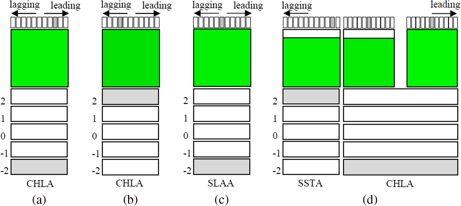

5. Case Study

The monthly SST, CHL, SLA, sea surface wind (the U-component of wind: UWnd, and V-component of wind: VWnd), and SSP products from remote sensing imagery, and the multivariate ENSO index (MEI) were used in this analysis. The temporal and spatial resolutions of the remote sensing imagery and the MEI are summarized in Table 2. An analysis period from January 1998 to December 2011 was selected. As Pacific Ocean was a more interactive region among marine environmental parameters and ENSO, playing an important role in both global climate change and regional sea–air interaction,²⁸^,²⁹ the area covering 100°E to 60°W and 50°S to 50°N was taken as the research area. The association rule mining algorithm based on the mutual information was applied, and the minimum dynamic supports, defined according to variation types, a confidence threshold of 75%, and a time distance of 12 months was set up, as used by Xue et al.²⁷

Table 2

Sources and resolution of remote sensing imagery used in this study.

	Product	Source	Time span	Temporal resolution	Spatial coverage	Spatial resolution
1	SST	NOAA/PSD	1981.12 to 2012.02	Monthly	Global	1° (Grid)
2	CHL	SeaWifs	1997.09 to 2010.11	Monthly	Global	9 km (Grid)
2	CHL	MODIS	2002.07 to 2012.03	Monthly	Global	4 km (Grid)
3	SSP	TRMM	1998.01 to 2011.06	Monthly	Global	0.25° (Grid)
4	Wind	CCMP	1987.07 to 2011.12	Monthly	Global	0.25° (Grid)
5	SLA	AVISO	1992.12 to 2011.12	Monthly	Global	1/3° (Mercator projection)
6	ENSO	MEI	1950.01 to 2012.03	Monthly	—	—

Note: SST, sea surface temperature; SSP, sea surface precipitation; SLA, sea level anomaly; ENSO, El Niño Southern Oscillation; MEI, multivariate ENSO index; NOAA/PSD, National Oceanic & Atmospheric Administration, Physical Sciences Division; TRMM, Tropical Rainfall Measuring Mission; CCMP, Cross-Calibrated Multi-Platform; AVISO, Archiving, Validation and Interpretation of Satellite Oceanographic data.

ArcGIS 10.0 is a prevailing commercial system consisting of several components, providing a scalable framework for managing, analyzing, and visualizing spatiotemporal data. ArcGeoDatabase is an object relational model for storing temporal and spatial graphical data, and ArcEngine is an embeddable GIS component library for building custom applications using multiple application programming interfaces. So, in this paper, we selected ArcGeoDatabase 10.0 to store the mined association patterns with the same structure as shown in Table 1 and designed interactive interfaces using ArcEngine 10.0 components for visualizing marine abnormal association patterns over scales ranging from global view to detailed.

The designed visualization components are DlgSTRulesVisualizationOnOverview, shown in Fig. 5, which produces a visualization interface giving an overview of regions of strong marine variation, DlgSTRulesVisualizationOn2DMap (Fig. 6), which represents the spatial distribution of the marine environmental parameter causing or responding to changes in others, and the DlgSTRulesVisualizationOnTripleLayerMosaics (Fig. 7) interface, which details the specified association patterns.

Fig. 5

Interface for overview of regions of strong marine variations.

Fig. 6

Interface for representing the spatial distribution of a specified marine parameter causing or responding to variations in other parameters.

Fig. 7

Interface for plotting the detailed association patterns. The color bar in the top map is the same as in Fig. 6.

It is not a straightforward task to plot the three-dimensional pie chart for all raster lattice points, so, for simplicity, this paper uses the number of antecedents or consequents in place of the specified parameters of the patterns occurring in each lattice point. When the parameters involved in the specific lattice point are needed, the three-dimensional pie charts are replotted according to the location of interest specified by the user. In Fig. 5, when the cursor moves over the Overview map, the row and column of the current location are shown in the Row and Column widget. Once the PlotPieChart button is clicked, the three-dimensional pie chart for the specified lattice point is plotted.

In Fig. 6, if we want to know where and how the specified marine parameter causes variations in other parameters, the Antecedent is selected, while if we want to know where and how the specified marine parameter responds to variations in others, the Consequent is selected. Figures 6(a) and 6(b) show the ENSO causes and responses for marine parameter variations, respectively.

Generally, Fig. 7 depends on Fig. 6. Once the Antecedent or Consequent is selected, the detailed triple-layer mosaics are easily plotted. For example, when the cursor moves to the 58th column and 60th row, the Row and Column widget will show their values. From Fig. 6, we know that in this lattice point a strong La Niña event controls the oceanic variation. When the TripleLayerMosaic button is clicked, only the association patterns caused by a strong La Niña event are plotted. The left, middle, and right mosaics represent the patterns $ENSO [- 2, 0] \to SLAA [2, (7 to 12)]$ (12.41%, 80.95%), $ENSO [- 2, 0] \to VWndA [- 2, (- 2 to 5)]$ (3.45%, 100%), and “ $ENSO [- 2, 0] \to SLAA [2, (7 to 12)] \to VWndA [- 2, (- 6 to - 4)]$ (3.45%, 100%), respectively.

6. Conclusions

Abnormal association patterns from multiple long-term marine raster datasets are difficult to visualize simultaneously because they are mined lattice point by point, and each lattice point has zero to many relationships among marine environmental parameters. This study aims to visualize a large number of such patterns and help to understand how, when, and where the marine environmental parameters in different regions co-drive or respond to the variations of the others against the background of global change. Starting from the description of the problem and the model representing the patterns, we design an interactive visualization framework with three complementary components to visualize marine abnormal patterns on scales ranging from the global view to a detailed view. The three-dimensional pie chart component identifies regions that show more or fewer interrelations between marine environmental parameters, together with the parameters involved. The two-dimensional variation maps component gives the spatial distribution of the marine environmental parameter variations that cause or respond to variations in others. The triple-layer mosaic plot component visualizes the detailed association patterns, including the parameters involved, variation types, evaluation indices, and temporal offset. As the remote sensing images with spatial information are input data, the proposed visualization framework was not limited to spatial constraints. That is to say, once the mined association patterns were stored in Geodatabase according to the predefined rules, we could visualize marine abnormal association patterns over scales ranging from global view to detailed using the designed visualization components.

Since it is a region sensitive to global change, the Pacific Ocean was taken as a study area, and a prototype system based on ArcEngine 10.0 was developed to test the effectiveness and efficiency of the visualization framework. For wide applications in real scenarios, we integrated the prototype system into the Marine Spatiotemporal Association Patterns Mining System (MarineSTAPMining), registered by national copyright administration of China with No. 2014SR013444. The MarineSTAPMining is developed by authors aiming at discovering and visualizing the spatiotemporal knowledge from large amount of remote sensing images. Its main functions include data pretreatment of long-term remote sensing images, design and implementation of mining algorithms, and spatiotemporal association patterns visualization. Compared with traditional visualization techniques that do not consider spatial information (textual form, table-based views, scatter plots, parallel coordinates plots, matrix, mosaic plots, and graph-based views), the complementary interactive visualization framework gives a strategy to visualize marine abnormal patterns from large to detailed scale according to the users’ request. Compared with visualization techniques using geospatial referencing,⁸^,²³ the proposed visualization framework not only visualizes the antecedents and consequents on the two-dimensional map, but also shows the detailed information for specified lattice point. While this proposed framework may be a promising tool for visualizing spatiotemporal association patterns in large raster datasets, we note that in our research work, only a few marine environmental parameters were involved, so it was easy to implement the three proposed complementary interfaces. Once a large number of marine environmental parameters are involved and the mined abnormal patterns contain many more parameters, the three-dimensional pie chart and two-dimensional variation map component will still simplify the visualization. However, it will not be so easy to visualize many groups of triple-layer mosaics or one triple-layer mosaic with multiple marine parameters for a specified lattice point vividly and intuitively in the triple-layer mosaic component.

Acknowledgments

This research was supported by the Fundamental Research Funds for the Central Universities (No. 13CX06012A), the National Natural Science Foundation of China (Nos. 41371385 and 41201399), the National High Technology Research and Development Program of China (No. 2012AA12A403-5), and the LREIS opening project.

References

1.

C. Wilson and D. Adamec, “Correlations between surface chlorophyll and sea surface height in the tropical Pacific during the 1997–1999 El Niño-Southern Oscillation event,” J. Geophys. Res., 106 (C12), 31175 –31188 (2001). http://dx.doi.org/10.1029/2000JC000724 JGREA2 0148-0227 Google Scholar

2.

R. Murtugudde et al., “Remote sensing of the Indo-Pacific region: ocean colour, sea level, winds and sea surface temperatures,” Int. J. Remote Sens., 25 (7–8), 1423 –1435 (2004). http://dx.doi.org/10.1080/01431160310001592391 IJSEDK 0143-1161 Google Scholar

3.

M. B. Uz and J. A. Yoder, “High frequency and mesoscale variability in SeaWiFS chlorophyll imagery and its relation to other remotely sensed oceanographic variables,” Deep Sea Res. Part 2 Top. Stud. Oceanogr., 51 (10–11), 1001 –1017 (2004). http://dx.doi.org/10.1016/j.dsr2.2004.03.003 0967-0645 Google Scholar

4.

G. Chen et al., “Seasonal-to-decadal modes of global sea level variability derived from merged altimeter data,” Remote Sens. Environ., 114 (11), 2524 –2535 (2010). http://dx.doi.org/10.1016/j.rse.2010.05.028 RSEEA7 0034-4257 Google Scholar

5.

M. Kahru et al., “Global correlations between winds and ocean chlorophyll,” J. Geophys. Res., 115 (C12), (2010). http://dx.doi.org/10.1029/2010JC006500 JGREA2 0148-0227 Google Scholar

6.

P. Tan et al., “Finding spatio-temporal patterns in earth science data,” (2014) ftp://ftp.cs.umn.edu/dept/users/kumar/spatio_temporal15.pdf May ). 2014). Google Scholar

7.

R. Hollmann et al., “The ESA Climate Change Initiative: satellite data records for essential climate variables,” Bull. Am. Meteorol. Soc., 94 (10), 1541 –1552 (2013). http://dx.doi.org/10.1175/BAMS-D-11-00254.1 BAMIAT 0003-0007 Google Scholar

8.

M. Bertolotto et al., “Towards a framework for mining and analysing spatio-temporal datasets,” Int. J. Geogr. Inf. Sci., 21 (8), 895 –906 (2007). http://dx.doi.org/10.1080/13658810701349052 1365-8816 Google Scholar

9.

V. Kumar, “Discovery of patterns in global Earth science data using data mining,” Lec. Notes Comput. Sci., 6118 2 (2010). http://dx.doi.org/10.1007/978-3-642-13657-3 LNCSD9 0302-9743 Google Scholar

10.

F. M. Hoffman et al., “Data mining in Earth system science (DMESS 2011),” Procedia Comput. Sci., 4 1450 –1455 (2011). http://dx.doi.org/10.1016/j.procs.2011.04.157 1877-0509 Google Scholar

11.

P. S. Zhang et al., “Discovery of patterns in the Earth science data using data mining,” Next Generation of Data Mining Applications, 167 –188 IEEE Press, Hoboken, New Jersey (2005). Google Scholar

12.

J. W. Lee and Y. J. Lee, “A knowledge discovery framework for spatiotemporal data mining,” Int. J. Inf. Process. Syst., 2 (2), 124 –129 (2006). Google Scholar

13.

T. S. Korting, L. M. G. Fonseca and G. Camara, “GeoDMA—Geographic Data Mining Analyst,” Comput. Geosci., 57 133 –145 (2013). http://dx.doi.org/10.1016/j.cageo.2013.02.007 1420-0597 Google Scholar

14.

R. J. Bayardo and R. Agrawal, “Mining the most interesting rules,” in Proc. of the Fifth ACM SIGKDD Int. Conf. on Knowledge Discovery and Data Mining, 145 –154 (1999). Google Scholar

15.

A. Inselberg and B. Dimsdale, “Parallel coordinates: a tool for visualizing multi-dimensional geometry,” in Proc. of the IEEE Conf. on Visualization, 361 –378 (1990). Google Scholar

16.

H. Hofmann, A. P. J. M. Siebes and A. F. X. Wilhelm, “Visualizing association rules with interactive mosaic plots,” in Proc. of the Sixth ACM SIGKDD Int. Conf. on Knowledge Discovery and Data Mining, 227 –235 (2000). Google Scholar

17.

H. Hofmann and A. Wilhelm, “Visual comparison of association rules,” Comput. Stat., 16 (3), 399 –416 (2001). http://dx.doi.org/10.1007/s001800100075 CSTAEB 0943-4062 Google Scholar

18.

G. Ertek and A. Demiriz, “A framework for visualizing association mining results,” Lec. Notes Comput. Sci., 4263 593 –602 (2006). http://dx.doi.org/10.1007/11902140 LNCSD9 0302-9743 Google Scholar

19.

A. Ceglar et al., “Visualising hierarchical associations,” Knowl. Inf. Syst., 8 (3), 257 –275 (2005). http://dx.doi.org/10.1007/s10115-003-0139-0 0219-1377 Google Scholar

20.

K. Techapichetvanich and A. Datta, “VisAR: a new technique for visualizing mined association rules,” in Proc. of the Int. Conf. on Advanced Data Mining and Applications, 88 –95 (2005). Google Scholar

21.

D. Bruzzese and C. Davino, “Visual mining of association rules,” Lec. Notes Comput. Sci., 4404 103 –122 (2008). http://dx.doi.org/10.1007/978-3-540-71080-6 LNCSD9 0302-9743 Google Scholar

22.

Y. A. Sekhavat and O. Hoeber, “Visualizing association rules using linked matrix, graph, and detail views,” Int. J. Intell. Sci., 3 (1A), 34 –49 (2013). http://dx.doi.org/10.4236/ijis.2013.31A005 IJISED 1098-111X Google Scholar

23.

P. Compieta et al., “Exploratory spatio-temporal data mining and visualization,” J. Vis. Lang. Comput., 18 (3), 255 –279 (2007). http://dx.doi.org/10.1016/j.jvlc.2007.02.006 JVLCE7 1045-926X Google Scholar

24.

J. Blanchard et al., “A 2D-3D visualization support for human-centered rule mining,” Comput. Graph., 31 (3), 350 –360 (2007). http://dx.doi.org/10.1016/j.cag.2007.01.026 0097-8493 Google Scholar

25.

K. E. Trenberth, “The definition of El Niño,” Bull. Am. Meteorol. Soc., 78 (12), 2771 –2777 (1997). http://dx.doi.org/10.1175/1520-0477(1997)078<2771:TDOENO>2.0.CO;2 BAMIAT 0003-0007 Google Scholar

26.

X. Y. Li and P. M. Zhai, “On indices and indictors of ENSO episodes,” Acta Meteorol. Sinica, 58 (1), 102 –119 (2000). 0894-0525 Google Scholar

27.

C. J. Xue, Q. Qing and X. Fan, “Spatiotemporal association patterns of multiple parameters in the northwestern Pacific Ocean and their relationships with ENSO,” Int. J. Remote Sens., IJSEDK 0143-1161 Google Scholar

28.

J. C. L. Chan, “Interannual and interdecadal variations of tropical cyclone activity over the western North Pacific,” Meteorol. Atmos. Phys., 89 (1), 143 –152 (2005). http://dx.doi.org/10.1007/s00703-005-0126-y MAPHEU 1436-5065 Google Scholar

29.

M. J. McPhaden, S. E. Zebiak and M. H. Glantz, “ENSO as an integrating concept in earth science,” Science, 314 (5806), 1740 –1745 (2006). http://dx.doi.org/10.1126/science.1132588 SCIEAS 0036-8075 Google Scholar

Biography

Lianwei Li is a lecturer in the College of Geoscience and Technology, China University of Petroleum, China. He received his MS degrees in human geography from East China Normal University in 2005 and achieved his PhD from China University of Petroleum. He is the author of 10 journal papers. His current research interests include object-oriented model and data mining.

Cunjin Xue is an associate professor at the Institute of Remote Sensing and Digital Earth, Chinese Academy of Sciences (CAS), China. He received his MS degree in GIS from Wuhan University in 2005 and his PhD degree in GIS from Institute of Geographical Sciences and Natural Resources Research, CAS. He is the author of more than 30 journal and proceeding papers. His current research interests include marine GIS and spatiotemporal mining algorithms.

Biographies of the other authors are not available.

CC BY: © The Authors. Published by SPIE under a Creative Commons Attribution 4.0 Unported License. Distribution or reproduction of this work in whole or in part requires full attribution of the original publication, including its DOI.

Citation Download Citation

Lianwei Li, Cunjin Xue, Jian Liu, Zhenjie Wang, and Lijuan Qin "Raster-based visualization of abnormal association patterns in marine environments," Journal of Applied Remote Sensing 8(1), 083615 (11 June 2014). https://doi.org/10.1117/1.JRS.8.083615

Published: 11 June 2014

Access the abstract

JOURNAL ARTICLE
13 PAGES

DOWNLOAD PAPER SAVE TO MY LIBRARY

GET CITATION

CITATIONS

Cited by 3 scholarly publications.

Explore citations on Lens.org

KEYWORDS

Visualization

Oceanography

Ocean optics

Raster graphics

Environmental sensing

Human-machine interfaces

Coastal modeling

1.

Introduction

2.

Challenges

Eq. (1)

3.

Association Pattern Representation Model

Property I:

Property II:

Table 1

Eq. (2)

4.

Interactive Visualization Framework

Fig. 1

4.1.

Three-Dimensional Pie Chart Component

Fig. 2

4.2.

Two-Dimensional Variation Map Component

Fig. 3

4.3.

Triple-Layer Mosaic Plot Component

Eq. (3)

Fig. 4

5.

Case Study

Table 2

Fig. 5

Fig. 6

Fig. 7

6.

Conclusions

Acknowledgments

References

Biography

Show All Keywords

Keywords/Phrases

Search In:

Publication Years