Point spread function of (multiple) Bracewell interferometric configuration(s) and the nulling hypothesis in planet detection

Marija Strojnik

doi:10.1117/1.JRS.8.084981

16 June 2014 Point spread function of (multiple) Bracewell interferometric configuration(s) and the nulling hypothesis in planet detection

Marija Strojnik

Author Affiliations +

Journal of Applied Remote Sensing, Vol. 8, Issue 1, 084981 (June 2014). https://doi.org/10.1117/1.JRS.8.084981

Abstract

We perform a rigorous, diffraction-based two-dimensional analysis to develop an analytical expression for the point spread function (PSF) of the multiple Bracewell interferometric (in-line, even-numbered multi-aperture) configurations proposed for extrasolar planet detection. The number of apertures, total length of interferometer array, and the diameter and shape of individual apertures control the PSF. We show that there are theoretically just a few points where the PSF is zero for monochromatic radiation. These zero-irradiance points disappear due to the spectral width of the source spectrum. When including, also, the finite spatial extend of the source, it is impossible to detect an image of a planet with just a two-aperture interferometer. This analysis further demonstrates that the so-called nulling interferometric techniques decrease the amount of detected radiation originating at the bright star by the same factor as that emitted by the planet.

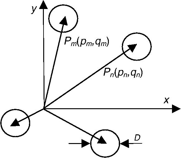
1. Interferometry for Star-Light Nulling

Approximately 35 years ago, a number of prominent scientists participated at a conference to discuss the detection of planets outside our solar system to set out the long-range plans for future planetary research. This scientific gathering resulted in a note in Nature, proposing the detection of nonsolar planets by free-spinning infrared (IR) two-aperture interferometer.¹ A new term, nulling, was coined to indicate that by a clever choice of interferometer parameters, its components, and configuration, the radiation emitted by the star could be cancelled (made to go away) at specific extended regions in the detection plane, in which the existence of a faint planet could thus be confirmed.²

We develop the analytical expression for the monochromatic incidence distribution in the observation plane arising from an IR point source at infinity, collected by a set of inline apertures with finite diameter, the monochromatic point spread function (PSF).³ In previous analysis, only point apertures have been considered.² We extend the discussion to include finite-diameter apertures to allow also collection of radiative power. This formal treatment represents a continuation of earlier analysis based on the Huygens’ principle.⁴

We find that the aperture separation, $L$ , in an interferometric layout approximately replaces the aperture diameter $D$ to identify the equivalent resolution angle, $0.75 λ / L$ , for the original Bracewell configuration. The separation between the outermost apertures, $L$ , replaces the aperture diameter, in the case of the multiple Bracewell configurations. The resolution along the perpendicular direction, corresponding to a single aperture, is $1.22 λ / D$ , with symbol $λ$ denoting wavelength.⁵

The objective of this work is to present theoretical development in support of the hypothesis that a simple, two-aperture interferometric system does not null the star light; but, rather, that both the star and the planet form an interferometric pattern each over the finite spatial region in the far plane.

2. Optical Transfer Function and the Point Spread Function

PSF or the impulse response function is the response of the optical system to the point input. It is a general system-level description of the performance of an optical instrument that includes the effects of diffraction. The PSF, given as a function of spatial coordinates in the image plane, is the image of the point object. When the point source is at infinity, as in the case of stars, the image is formed in the focal plane at a distance $f$ behind the aperture plane. The Fourier transform of the PSF is, in general, a complex function referred to as the optical transfer function (OTF). The Fourier transform of the image may then be found by multiplying the Fourier transform of the object by the OTF. In the spatial domain, the image may be obtained as a two-dimensional (2-D) convolution (denoted as **) of the object function with the PSF, involving a set of mathematical operations in complex domain.

2.1.

Aperture Function

We begin the theoretical development by defining the generalized pupil function. A general pupil may consist of $N$ subapertures, centered at $P_{n} (p_{n}, q_{n})$ ,

Eq. (1)

P (r) = \sum_{n = 1}^{N} W_{D} (r - P_{n}) .

Here, we use the vector notation as a shortcut for writing out the components, i.e., $r = (x, y)$ , and $r = | r |$ is the magnitude of the radial coordinate in the aperture plane. The single circular aperture function of diameter $D$ , centered at the origin, $W_{D} (r)$ , may be represented as a one-zero radial step function:

Eq. (2)

W_{D} (r) = circ (\frac{| r |}{D / 2}) = {\begin{matrix} 1 & when & | r | / D \leq 1 / 2 \\ 0 & when & | r | / D > 1 / 2 \end{matrix} .

The aperture function in Eq. (1) may be rewritten as follows, upon the substitution of Eq. (2):

Eq. (3)

P (r) = circ (\frac{| r |}{D / 2}) * * \sum_{n = 1}^{N} δ (r - P_{n}) .

This pupil function is illustrated in Fig. 1. The aperture distribution breaks the circular symmetry of the problem, making the use of the Cartesian coordinates more convenient for a multiple aperture system. The amplitude impulse response $P (U)$ of a coherent optical system is the 2-D Fourier transform, $F {}$ , of the aperture distribution function, given in Eq. (3), $F {P (r)}$ . The Fourier transform of a function of spatial coordinates $(r) = (x, y)$ is given in $(U) = (U, V)$ coordinates.

Fig. 1

Geometrical parameters for a two-dimensional (2-D) layout of circular apertures.

The PSF, $h (U)$ , of an incoherent system, such as the ones considered here that employ the IR radiation to carry the information, is a square of the response of the coherent one.

Eq. (4)

h (U) = {| F {P (r)} |}^{2} = [F {P (r)}] {[F {P (r)}]}^{*} .

The symbol * denotes the complex conjugate. The (in)coherent PSF may also be given in terms of the spatial coordinates in the image plane, $(x_{i}, y_{i})$ , when the spatial frequency domain coordinates $U$ are replaced by $π r_{i} D / λ f$ . Subscript $i$ denotes image quantities. The distance between the aperture plane and the image plane is $f$ , often the focal distance of an imaging instrument. The OTF is the 2-D Fourier transform of the PSF:

Eq. (5)

OTF (f_{x}) = F {h (U)} = F {{| F {P (r)} |}^{2}} = F {| [F {P (r)}] {[F {P (r)}]}^{*}} .

The Fourier transform of the product of two Fourier-transformed (pupil) functions is also the convolution of the pupil functions, expressed as a function of the Fourier space coordinates (inverse distances, in this case). When the pupil function is a simple zero-one function (a particularly simple case of a real function), it is also its own complex conjugate.

Eq. (6)

OTF (f_{x}) = F {[F {P (r)}]} ** F {[F {P (r)}] *} = P (f_{x}) ** P (f_{x}) .

Here, $f_{x}$ denotes the spatial frequency coordinates, or more specifically, the coordinates in the Fourier space. In the special case that the PSF arises solely upon diffraction at a (set of) clear aperture(s), the $OTF (f_{x})$ may easily be found as a convolution of the aperture transmission function with itself. The general aperture distribution of Fig. 1 is one such case when the convolution may be performed appropriately.

We may formulate the PSF in the image space, denoted $h (x_{i,} y_{i})$ , starting from the aperture function. First, we find the amplitude PSF (APSF), denoting it $η (x_{i,} y_{i})$ , the not yet normalized PSF. Taking the Fourier transform of Eq. (3), we recall that the Fourier transform of a convolution of two functions is a product of the Fourier transform of individual functions:

Eq. (7)

η (x_{i,} y_{i}) = J {circ (\frac{| r |}{D / 2})} J {\sum_{n = 1}^{N} δ (x - p_{n}, y - q_{n})} | \begin{matrix} U = (π x_{i} D / λ f) \\ V = (π y_{i} D / λ f) \end{matrix} .

The right side of Eq. (7) may be further simplified upon finding the Fourier transform of each function in the product. The APSF, $η (x_{i}, y_{i})$ , then becomes

Eq. (8)

η (x_{i}, y_{i}) = {\frac{2 J_{1} [{(U^{2} + V^{2})}^{1 / 2}]}{{(U^{2} + V^{2})}^{1 / 2}}} {\sum_{n = 1}^{N} \exp [- i 2 (U p_{n} + V q_{n}) / D]} | \begin{matrix} U = (π x_{i} D / λ f) \\ V = (π y_{i} D / λ f) \end{matrix} .

The Fourier transform of the aperture function for the pupil of diameter $D$ is equal to twice the Bessel function of the first order, divided by its argument. In astronomy, it is customary to replace the distances in the plane of detection $(x_{i}, y_{i})$ with the angular coordinates $(U, V)$ . The phase in each exponential function, $Φ_{n} (p_{n}, q_{n})$ , is the optical path (delay) between a wave originating at the center of the $n$ ’th aperture at $(p_{n}, q_{n})$ relative to the one at the origin.⁵

Eq. (9)

Φ_{n} (p_{n}, q_{n}) = - 2 (U p_{n} + V q_{n}) / D = - 2 π (x_{i} p_{n} + y_{i} q_{n}) / λ f .

The phase difference of the radiation, collected by the $P_{n} (p_{n}, q_{n})$ ’th and $P_{m} (p_{m}, q_{m})$ ’th apertures, diffracted there, and observed in the image plane at the point $(x_{i}, y_{i})$ in this expression, is determined primarily by the aperture location. The specific position on each aperture impacts it secondarily, although it contributes to the shape of the PSF.

2.2.

Equidistant Apertures in a Line

Equation (8) may be evaluated in a closed form for the case of a redundant, linear array of $N$ equally spaced apertures, when $N$ is even (see Fig. 2, a double Bracewell configuration). The term redundancy refers to the fact that more than one subaperture pair samples a particular spatial frequency. The center-to-center separation of adjacent apertures is $γ D$ , with $γ > 1$ to prevent the aperture overlap. We propose to refer to $γ$ as one-dimensional dilution factor

Eq. (10)

γ = L / [D (N - 1)] .

Fig. 2

The simplest case of multiple Bracewell interferometric configurations: a linear array with four apertures of diameter $D$ . The center-to-center separation of adjacent apertures is $γ D$ ; the center-to-center separation between extreme apertures is 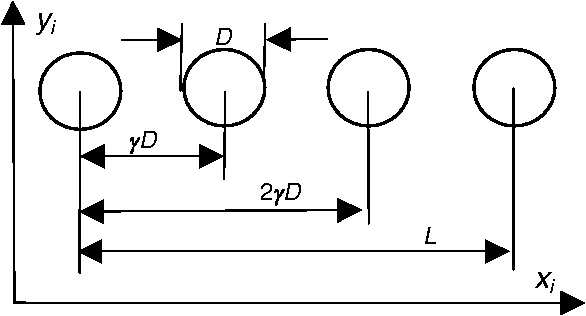$L$ .

The subaperture centers are located on x-axis, at positions $p_{n} = \pm γ D / 2, \pm 3 γ D / 2, \dots, \pm (2 N - 1) γ D / 2$ measured from the array center. The total distance spanned by the array of $N$ apertures is $[(N - 1) γ D + D]$ . The distance $L = (N - 1) γ D$ is the center-to-center separation of the extreme apertures. The finite sum in the second factor in Eq. (8) may be evaluated for the inline apertures, yielding a real-valued (rather than complex) analytical result:

Eq. (11)

\sum_{n = 1}^{N} \exp [- i 2 (U p_{n} + V q_{n}) / D] = 2 \sum_{n = 1}^{N / 2} \cos [(2 n - 1) γ U] = \frac{\sin (N γ U)}{\sin (γ U)} = \frac{\sin [N (γ π x_{i} D) / (λ f)]}{\sin [(γ π x_{i} D) / (λ f)]} .

After substituting the expression in the third equality of Eq. (11) into Eq. (8), the APSF of a linear array of equidistant apertures is found:

Eq. (12)

η (x_{i}, y_{i}) = {\frac{2 J_{1} [{(U^{2} + V^{2})}^{1 / 2}]}{{(U^{2} + V^{2})}^{1 / 2}}} {\frac{\sin (N γ U)}{\sin (γ U)}} | \begin{matrix} U = (π x_{i} D / λ f) \\ V = (π y_{i} D / λ f) \end{matrix} .

This expression may be written out as follows, after the variables for the spatial frequency coordinates have been substituted:

Eq. (13)

η (x_{i}, y_{i}) = {\frac{2 J_{1} [{(x_{i}^{2} + y_{i}^{2})}^{1 / 2} (π D / λ f)]}{\begin{matrix} {(x_{i}^{2} + y_{i}^{2})}^{1 / 2} (π D / λ f) \end{matrix}}} {\frac{\sin [N (γ π D x_{i}) / (λ f)]}{\sin [(γ π D x_{i}) / (λ f)]}} .

The PSF of the incoherent optical system, $h (x_{i}, y_{i})$ , is the square of the APSF normalized to 1 at the origin. Using the L’Hôpital rule, we may find its value at the origin to be equal to $N$ . We first square the right side of Eq. (12), and then normalize it by its value at the origin, $N^{2}$ . Physically, this means that $N$ apertures collect $N$ times the radiative power of a single aperture.

Eq. (14)

h (U, V) = \frac{1}{N^{2}} {[\frac{2 J_{1} {(U^{2} + V^{2})}^{1 / 2}}{{(U^{2} + V^{2})}^{1 / 2}}]}^{2} {[\frac{\sin (N γ U)}{\sin (γ U)}]}^{2} | \begin{matrix} U = (π x_{i} D / λ f) \\ V = (π y_{i} D / λ f) \end{matrix} .

Both functions in this expression are decreasing with the increasing argument, up to the first zero of the Bessel and sine-square functions, respectively. The zeros of the Bessel function along the $U$ -axis occur for values, $U_{0 B} = 1.220 π, 2.233 π, 3.238 π, \dots$ The primary maxima of the multiple-beam interference function take place at angles, $U_{IM}$ .

Eq. (15)

U_{IM} = m [λ / (D γ)] = m [(N - 1) (λ / L)] for integers m = 1, 2, 3, 4, \dots

The zeros, $U_{0 I}$ , are present for all values of integer $n$ , except where the maximum occurs.

Eq. (16)

U_{0 I} = n [λ / (DN γ)] = n {[(N - 1) / N] (λ / L)} for integers n = 1, 2, 3, 5, 6, 7, 9, 10, 11, 13 \dots .

The zeros of the sine function occur for smaller values of $U$ than those of the Bessel function of the first order, as a consequence of the physical necessity that the interferometer linear distance $L$ be larger than the aperture diameter $D$ . Therefore, the PSF, Eq. (14), may be interpreted as the second term (square of the sine function), modulating the first factor (square of the Bessel function). The primary effect of interference is rapid signal attenuation for off-axis image coordinates. The signal attenuation is also a physical consequence of the finite total aperture area that determines the amount of collected light.

We may substitute the actual values for $U$ and $V$ , or use Eq. (13), to express this result for the PSF in terms of the spatial coordinates in the interference plane:

Eq. (17)

h (x_{i}, y_{i}) = \frac{1}{N^{2}} {\frac{2 J_{1} [{(x_{i}^{2} + y_{i}^{2})}^{1 / 2} (π D / λ f)]}{[{(x_{i}^{2} + y_{i}^{2})}^{1 / 2} (π D / λ f)]}}^{2} {\frac{\sin [N (γ π D x_{i} / λ f)]}{\sin [(γ π D x_{i} / λ f)]}}^{2} .

Thus, we have derived an analytical expression for the PSF of a set of $N$ apertures, with $N$ even, and aperture diameter $D$ , either in terms of $(U, V)$ angular coordinates [Eq. (14)] or spatial coordinates in the image plane, $x_{i}$ , $y_{i}$ , [Eq. (17)].

3. First Zero of the Point Spread Function

We next examine the resolution of arrays with finite aperture diameter, considering that the resolution (distance) corresponds to the distance from the coordinate origin to the first zero of the PSF. We keep in mind that high resolution corresponds to short distance.

The following parameters were chosen for the simulation study. The separation of centers of two edge apertures, $L$ , is 10 m; there are four apertures ( $N = 4$ ), and the aperture diameter, $D$ , is 1 m. These values uniquely specify the normalized aperture separation in terms of the aperture diameter, $γ$ , ( $10 / 3$ ). Figure 3 shows the PSF of the linear configuration as a function of the normalized angle $U$ coordinate, $U / π$ , for $V = 0$ . Furthermore, this variable may be replaced by $π x_{i} D / λ f$ , hence the PSF or the normalized incidence for a point input may also be given as a function of the spatial coordinates in the image detection plane.

Fig. 3

Point spread function as a function of angle $U / π$ for the double Bracewell configuration (four equidistant circular apertures, in a line). The following parameters were used to generate the graph: baseline $L$ is 10 m, aperture diameter $D$ is 1 m, and the aperture separation in units of aperture diameter, $γ$ , is equal to $10 / 3$ . The angle subtended between the central peak and the first minimum is 0.75 ( $λ / L$ ).

The PSF graph illustrates that the first two side lobes have small amplitude, similar to the case of a single aperture. However, the third and the sixth side lobes are somewhat pronounced. The two small side lobes surrounding the central peak enhance it and delineate its narrow spatial extent along the $U$ -coordinate. Along the perpendicular $V$ direction, the PSF is equal to that of a single aperture (see Ref. 5).

Both factors on the right side of Eq. (14) decrease as a function of their argument, up to their respective first zero. However, the multiple-beam interference function attains zero value for the lower values of the focal plane coordinates ( $0.75 λ / L$ ) than the Bessel function of the first order ( $1.22 λ / D$ ), the Rayleigh single-aperture angular resolution. The interferometer array length, $L$ , and the aperture diameter, $D$ , determine this angle, for the same wavelength of observation.

4. First Zero of a Single-Aperture System

The Rayleigh resolution of a single aperture of diameter $D$ is equal to one-half the width of the Airy disk, $r_{i 0} = 1.22 λ f / D$ . Its value is found when the Bessel function of the first order is equal to zero for the smallest value of its argument. The angular resolution of a single aperture of diameter $D$ , $α_{r}$ , is the Rayleigh resolution distance divided by the focal length $f$

Eq. (18)

α_{r} = r_{i 0} / f = 1.22 λ / D .

4.1.

First Zero of a Multiple, Even-Numbered Aperture System

We may define the angular resolution of an interferometric array in a manner analogous to that of the Rayleigh resolution limit. It is the smallest absolute value of the angular coordinate $U$ for which the incidence drops to zero, divided by the focal distance. Dealing with the position coordinate in Eq. (17), the zero value of incidence is found when the argument of the sine function in the numerator, $U = (N γ π x_{i} D) / (λ f)$ , is equal to $π$

Eq. (19)

x_{i 0} = (λ f) / (N γ D) = [(N - 1) / N] (λ f / L) .

After substituting for $γ$ , we find the equivalent resolution along the line of apertures. Interestingly, the resolution is improved for a given number and diameter of apertures when their separation is increased. The angular resolution of $N$ equidistant apertures along line $L$ , $α_{i 0}$ , is the spatial resolution, divided by the focal length $f$

Eq. (20)

α_{x i} = x_{i 0} / f = (λ) / (DN γ) = [(N - 1) / N] (λ / L) .

The first factor in the third equality increases from $0.5 (= 1 / 2)$ to $3 / 4, 5 / 6, 7 / 8, \dots$ approaching asymptotically to 1 when number of apertures, $N$ , increases. The aperture diameter of the Rayleigh resolution is approximately replaced by $DN γ$ . The maximum value for the angular resolution for two apertures in contact is $0.5 λ / D (= 0.5 λ / L)$ . With increasing number of apertures $N$ in contact, the asymptotic maximum value for the resolution $α_{r \max}$ becomes $λ / (ND)$ , approximately $N$ times better (smaller) than that of a single aperture with the same diameter. However, it decreases as the aperture separation increases. We keep in mind the linguistic difficulty involved with the concept of resolution: it is better or higher when its numerical value is smaller.

Examining the second equality in Eq. (20), we note that the resolution of a multiple-aperture system is actually independent of the aperture diameter. The length of the inline equidistant aperture array approximately replaces the aperture diameter in the equivalent resolution expression.

4.2.

First Zero of the Bracewell Configuration (Two-Aperture System)

We evaluate the location of the first zero of a two-aperture interferometric system by setting $N$ to 2. Dealing with the position coordinate in Eq. (17), the zero value of incidence is found when the argument of the sine function in the numerator, $(2 γ π x_{i} D) / (λ f)$ , is equal to $π$ . From Eq. (19) we find

Eq. (21)

x_{i 0} = (λ f) / (N γ D) = (1 / 2) (λ f / L) .

The angular resolution of two equidistant apertures along line $L$ , $α_{i 0}$ , is the spatial resolution, divided by the focal length $f$

Eq. (22)

α_{x i} = x_{i 0} / f = (λ) / (2 γ D) = (1 / 2) (λ / L) .

The value for resolution $α_{x i}$ becomes $λ / (2 L)$ , approximately one-half that of a single aperture when apertures are in contact. It also improves with an increasing interaperture separation.

5. Conclusions

We developed theory in support of the hypothesis that simple, two-aperture interferometric system does not “null” the star light and, furthermore, that both star and planet form an interferometric pattern in a finite spatial region in the far plane.

The length of the inline two apertures layout effectively replaces the aperture diameter in the equivalent resolution expression, for the double Bracewell configuration. The resolution along the perpendicular direction is that of a single aperture.

The number of points in which the incidence due to a point source at infinity is zero for a four-aperture light-collection system is small, less than 10, within the field of view of the collector system. The incidence distribution due to a spectral star, an extended body emitting radiation within a spectral interval, located in infinity includes no points of zero incidence within the field of view of the instrument. Likewise, the incidence distribution in the observation plane due to a planet has a similar finite extend, covering about the same region of space as that originating at the star. This makes it impossible to plan for the planet image location at a preselected point in the image plane.

According to this theoretical analysis, there are no points in the far-field plane of the multiple-aperture array where the star radiation might be nulled. Thus, a more sophisticated instrument may need to be devised to enhance planetary attributes in the presence of its high-brightness star.⁶^,⁷

Acknowledgments

The CONACYT, the Mexican Science Foundation, provided funding to perform this work.

References

1.

R. N. Bracewell, “Detection of nonsolar planets by spinning infrared interferometer,” Nature, 274 780 –781 (1978). http://dx.doi.org/10.1038/274780a0 NATUAS 0028-0836 Google Scholar

2.

O. P. Lay, “Systematic errors in nulling interferometers,” Appl. Opt., 43 (33), 61006123 (2004). http://dx.doi.org/10.1364/AO.43.006100 APOPAI 0003-6935 Google Scholar

3.

M. StrojnikG. Paez, “Radiometry,” Handbook of Optical Engineering, 649 –700 Marcel Dekker, New York (2001). Google Scholar

4.

C. Vazquez-JaccaudM. StrojnikG. Paez, “Effects of a star as an extended body in extra-solar planet search,” J. Mod. Opt., 57 (18), 1808 –1814 (2010). http://dx.doi.org/10.1080/09500340.2010.528564 JMOPEW 0950-0340 Google Scholar

5.

G. PaezM. Strojnik, “Telescopes,” Handbook of Optical Engineering, 207 –226 Marcel Dekker, New York (2001). Google Scholar

6.

M. StrojnikG. PaezM. Mantravadi, “Lateral shearing interferometry,” Optical Shop Testing, 649 –700 Marcel Dekker, New York (2007). Google Scholar

7.

M. S. Scholl, “Signal detection by an extra-solar-system planet detected by a rotating rotationally-shearing interferometer,” J. Opt. Soc. Am. A., 13 (7), 1584 –1592 (1996). http://dx.doi.org/10.1364/JOSAA.13.001584 JOAOD6 1084-7529 Google Scholar

Biography

Marija Strojnik received her MS degrees in physics, optical sciences, and engineering, and her PhD degree in optical sciences. NASA awarded her six technology development certificates. She conceptualized, designed, and demonstrated an autonomous, star-pattern-based navigation technique, employing an intelligent camera, for in situ navigation decisions. This discovery is described in the popular Through the Wormhole TV program. SPIE conferred upon her the George W. Goddard award. She is a fellow of the OSA and SPIE.

CC BY: © The Authors. Published by SPIE under a Creative Commons Attribution 4.0 Unported License. Distribution or reproduction of this work in whole or in part requires full attribution of the original publication, including its DOI.

Citation Download Citation

Marija Strojnik "Point spread function of (multiple) Bracewell interferometric configuration(s) and the nulling hypothesis in planet detection," Journal of Applied Remote Sensing 8(1), 084981 (16 June 2014). https://doi.org/10.1117/1.JRS.8.084981

Published: 16 June 2014

Access the abstract

JOURNAL ARTICLE
8 PAGES

DOWNLOAD PAPER SAVE TO MY LIBRARY

GET CITATION

CITATIONS

Cited by 7 scholarly publications.

Explore citations on Lens.org

KEYWORDS

Point spread functions

Interferometry

Planets

Fourier transforms

Stars

Spatial resolution

Interferometers

1.

Interferometry for Star-Light Nulling

2.

Optical Transfer Function and the Point Spread Function