|
|
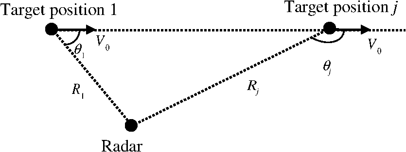
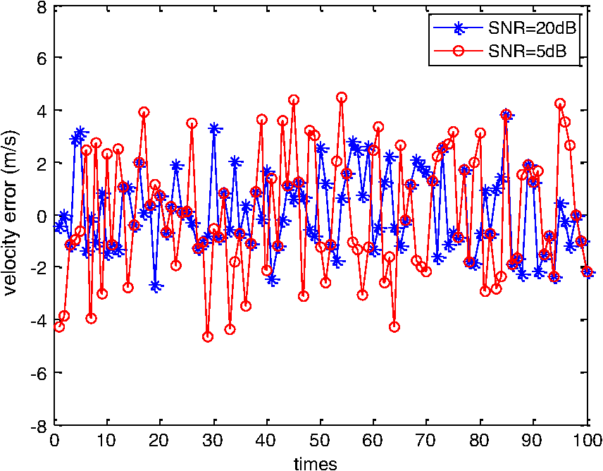
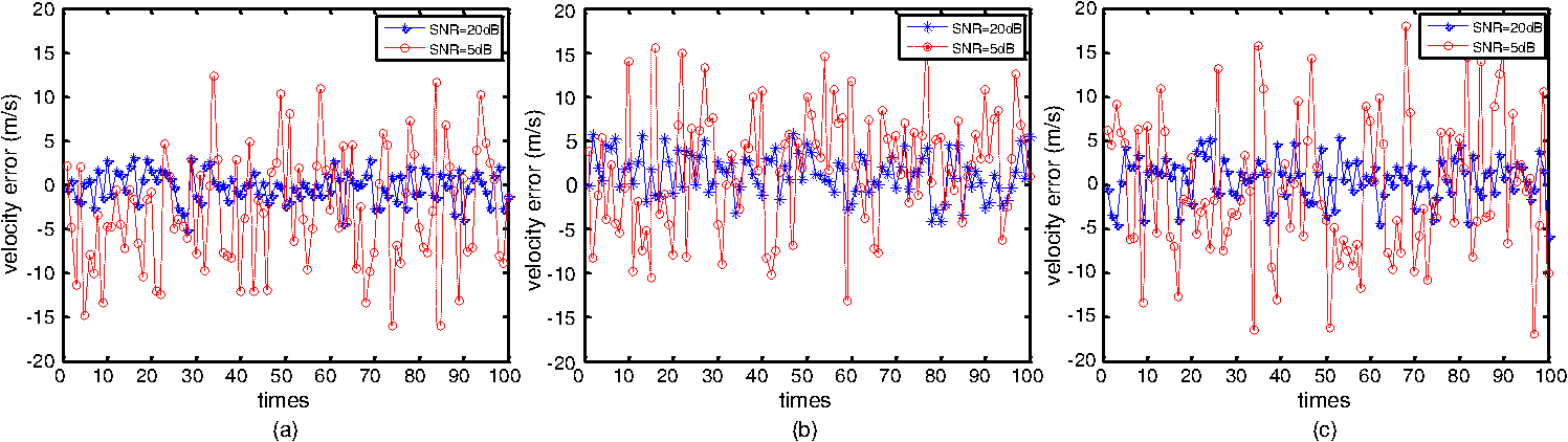
1.IntroductionTo meet the requirements of high-resolution range measurement or imaging, a step frequency technique has been proposed and has already become an important approach for modern radar systems. Stepped-chirp signal (SCS) has been a widely prevalent signal waveform used in synthetic aperture radar (SAR)/inverse SAR (ISAR).1–3 However, there exists a severe rang-Doppler coupling problem for SCS when applied to high-speed target imaging or detection. Because SCS is very sensitive to the radial velocity of target,4–7 the synthesized range profile suffers from range migration, energy diffusion, and resolution degradation, and even becomes meaningless if the motion compensation is not well done for high-speed target. So motion compensation is a crucial step in signal processing in this regard. There is a lot of research in this area and many methods for velocity measurement using SCS have been proposed, including the maximum likelihood method,8,9 iterative search method,10–12 pulse-Doppler (PD) auxiliary method,13 up-down stepped-chirp method,14–16 cross-correlation between frames method,17,18 etc. However, each of the above-mentioned methods has its limitations, such as the maximum likelihood method and iterative search method need a large amount of computation, the PD auxiliary method and up-down stepped-chirp method need an additional transmitting signal besides SCS, the cross-correlation between frames method needs high pulse repeat frequency (PRF) to obtain high measurement accuracy, etc. Recently, a preferable method named the cross-correlation inner frame method (CCIFM) was proposed.19 It can measure the radial velocity of a high-speed target without using an auxiliary signal in a low PRF situation and has the advantages of a small amount of computation and a large unambiguous measurement range. Although the measurement accuracy is not the highest among these methods, it still satisfies the requirement for motion compensation. The outstanding disadvantage of CCIFM is that it is only suitable for a single-scattering-center (SSC) target. In this paper, we extend the idea of cross-correlation inner frame and propose a new velocity measurement method, which is named the SCS multiple cross-correlation method (SCS-MCCM). As will be shown later, the SCS-MCCM can keep the advantages of CCIFM while overcoming its disadvantages. It focuses on the velocity measurement for a high-speed target in a much more practical situation, i.e., the multiple-scattering-center (MSC) target is considered. In the following section, the property of correlations between two paired subpulses in the SCS burst is extensively investigated with detailed formulas derived. It is demonstrated that the instantaneous radial velocity information can be extracted from each echo burst. Simulations show that the proposed approach performs very well on radial velocity estimate for a high-speed MSC target. Based on the measured velocity, motion compensation is conducted and high-resolution imaging of a high-speed MSC target is realized. Besides the radial velocity, the real target velocity can also be measured by the SCS-MCCM, which is very helpful for target identification. This is another superiority of the SCS-MCCM compared to other methods. 2.CCIFMThe transmitted waveform consists of a series of chirp pulses (subchirps or subpulses), whose carrier frequencies increase (or decrease) pulse by pulse in a step of . If the initial distance between radar and the target is , the radial target velocity is , and the pulse repeat interval is , then the time delay of the ’th subpulse is The echo of the ’th subpulse after being coherently received is where is the baseband chirp pulse, is the carrier frequency of the first pulse, is the frequency step, is the slope of the subpulse, is the subpulse time duration, , and is the number of subpulses in a burst. In the following, we ignore because it has no significant role in the derivation, as will be shown in the following. After cross-correlation processing on two subpulses spaced by subpulses, we can getEquation (3) shows that contains four terms: the first three terms are constant phases and the last term is a linear item of , which indicates a frequency shift. According to Eq. (3), the Doppler frequency of a moving target can be formulated as19 which is proportional to . So the target’s velocity can be measured by fast Fourier transform (FFT) of . The velocity measurement accuracy is related to the resolution of Doppler frequency. If we increase the FFT dots to by zero-padding, the minimum measurable velocity is then while the velocity measurement scope isNow, we shall show why can be ignored in Eq. (3) in detail as follows. We can easily obtain the following expression: For argument , the first three terms in Eq. (7) are constant phases and the last term is a linear item, which indicates a frequency, i.e., Generally speaking, is much smaller than , and the ratio is usually , so it can be ignored. 3.SCS-MCCMWhen the target is complex with MSCs, the correlation signals become much more complicated. Let us assume the number of scattering centers is ; the echo of the ’th subpulse is thus Because is the sum of echoes from scatterers, the correlation signals will have self-terms (self-correlation of the same scatterer’s echo) and cross-terms (cross-correlation of two different scatterers’ echoes), which lead to different frequency shifts. Therefore, we cannot estimate the velocity just by FFT as is done in Sec. 2. The cross-correlation between and is formulated as whereAmong the above phase terms, , , and are constant phases, , , , and are constant phases related to , and are linear items about , and , , , and are linear items about . As is shown, there are no coupling items about and . So, has terms, including self-terms(when ) and cross-terms(when ), which have different linear coefficients. That means the two-dimensional (2-D) spectrum of has many frequency components, and each of them corresponds to a self-term or a cross-term of . For self-terms, , , , , and do not exist. As is very small, as has been discussed previously, it can be ignored. With the constant phases , , and further ignored, we get Let represent the frequency along the direction and represent the frequency along the direction. Because (the linear item about ) and (the linear item about ) are not related to the scatterer’s position , and of the self-terms should be the same, and they are denoted as and , respectively. The cross-terms have different and different , which are related to the relative positions of scattering centers . As shown in Eq. (12), is decided by and , and is decided by , , and , i.e., From Eqs. (15) and (16), we can see that and are symmetrical pairs about and , respectively. When is less than a frequency resolution cell, i.e., , we can have . In this situation, the target can be regarded as a point target, so the velocity can be measured using the algorithm mentioned in Sec. 2. It means that the size of target should meet the requirement of , which is usually not satisfied in practical situations. That is to say the performance of the algorithm of Sec. 2 cannot be as good as we expect for bigger targets. In fact, we can also see from Eqs. (15) and (16) that the frequencies of cross-terms and are determined not only by , but also by . However, from Eqs. (13) and (14), we can see that the frequencies of self-terms and are determined only by . Therefore, if we can differentiate them in the 2-D spectrum of , the velocity can then be estimated by and . If a signal is sampled at rate and the sampling length is , then the resolution of the spectrum is . When , i.e., the distances between scattering centers of the target satisfy the following condition: After performing FFT on along the direction, and will be at least one frequency cell apart, so they can be easily distinguished. In fact, Eq. (17) is easy to meet via increasing by interpolation. Since is symmetrically distributed around , we can just choose the central frequency of the spectrum to get rid of all other frequency components of the cross-terms. At the last step, we get by conducting FFT along the direction and, finally, obtain the velocity by where . It is clear from Eq. (18) that the larger the , the higher the measurement accuracy but the less the unambiguous measurement range of velocity. We must choose an appropriate to balance the measurement range and accuracy. In fact, we can use a smaller to conduct a coarse measurement with a large unambiguous range first and then use a larger to conduct an accurate measurement.Figure 1 presents the flow chart of the proposed method, including the motion compensation step. The first step is to calculate a series of cross-correlations between two paired subpulses spaced by subpulses (, ; the second step is to perform FFT on the correlation signals along the direction for , ; the third step is to take the central spectral line of each pair to form a vector; the fourth step is to perform FFT on the above vector; the fifth step is to find the frequency corresponding to the peak value of the spectrum; the sixth step is to calculate the radial velocity according to Eq. (18); the seventh step is to conduct motion compensation according to the obtained velocity; the last step is to coherently synthesize the spectrums of all subpulses using the algorithm of Ref. 20 and, finally, get the high-resolution range profile through Inverse FFT (IFFT). 4.Real Velocity MeasurementIn this section, we shall show that besides the radial velocity, SCS-MCCM can also be used to measure the real velocity of the target. SCS-MCCM measures the radial velocity from the echoes of subpulses within a burst, i.e., it measures the instantaneous radial velocity at each burst. Then the real velocity can be estimated by combining the radial velocity measurement with the range measurement. Here, the target is supposed to be well tracked by radar. We assume that the target moves straight during the observation time, as shown in Fig. 2. The real target velocity is . When the radar is transmitting the ’th burst (), the distance between radar and target is , and the angle between the target moving direction and radar boresight is , so the radial velocity is ( is positive when and negative when ). If the burst repeat interval is , then the distance between target position 1 and target position is . According to the cosine law, we can get Eqs. (19) and (20), respectively, as follows: By substituting into Eq. (19), we can get By substituting into Eq. (20), we can get Finally, can be derived simultaneously from Eqs. (21) and (22). Equation (23) indicates that the real velocity measurement can be easily obtained by using the results of the range measurement as well as the radial velocity measurement, where the range measurement can be done according to the time delay of the radar echoes. In the following, let us analyze the impact of measurement errors of and on estimation. The measurement error (or accuracy) of , i.e., , can be formulated as follows: where and are the measurement errors of and , respectively. Equation (24) shows that when and are fixed (as discussed above), the smaller the partial derivatives with respect to and , the smaller the measurement error of , i.e., the higher the measurement accuracy of .The partial derivatives of Eq. (23) with respect to and , respectively, are as follows: In Eqs. (25) and (26), when , is positive. Along with the increase in , becomes larger, while and become smaller, so is positive and becomes larger, too; thus, the absolute values of and both become smaller. When , is negative, and its absolute value becomes larger as increases. Along with increase in , and also become larger, so is still positive and becomes larger, too; once again, the absolute values of and both become smaller. From the above analysis, we observed that the larger the , the smaller and . Therefore, in order to achieve high measurement accuracy of , we should choose a as large as possible. 5.SimulationsThe simulation parameters are as follows: , , , , , . Monte-Carlo simulations are conducted 100 times when the target velocities are produced with a uniform distribution in (, ). For the SSC target, CCIFM and SCS-MCCM have the same performance for the velocity measurement. Figure 3 presents the error curves of the velocity measurements for the SCC target with different SNRs. Results show that in the case of , the maximum measurement error is , while in the case of , the maximum measurement error is . That is to say the measurement error does not change significantly as the SNR decreases, i.e., MCCM exhibits a satisfied antinoise performance for the SSC target. Figures 4(a) and 4(b) present the high-resolution range profiles without and with motion compensation, respectively. When the target is moving at a high speed, the motion-induced phase errors will lead to image displacement and the image will be out of focus; therefore, high resolution cannot be achieved, as clearly shown in Fig. 4(a). Figure 4(b) shows that after velocity measurement and motion compensation, the burst of stepped-chirp can be synthesized correctly and a high-resolution range profile is, thus, obtained. The resolution in Fig. 4(b) is , which is close to the theoretical value of a 2.04-GHz bandwidth signal. In the following, we shall demonstrate the good performance of the SCS-MCCM for an MSC target. Figure 5 gives the MSC target model used for the velocity measurement and imaging simulations, which is composed of 41 ideal point targets. Fig. 4The synthesized range profiles for SSC target (a) without motion compensation and (b) with motion compensation.  We conduct Monte-Carlo simulation 100 times as before for the MSC target of Fig. 5 by using CCIFM with an and plot the obtained velocity measurement errors in Fig. 6, from which one can clearly see that they are very large and fluctuate dramatically. It means that CCIFM breaks down for the MSC target velocity measurement. Figure 7 presents the error curves of the velocity measurement by SCS-MCCM for the same MSC target with different SNRs. The target velocities in Figs. 7(a), 7(b), and 7(c) are varied in the range of (, ), (, ), and (, ), respectively. We can see from Fig. 7 that the measurement errors of the SCS-MCCM do not change as the target velocity changes, and they are all within when , while the maximum measurement errors are when . Compared to the SSC target case, the measurement accuracy for the MSC target degrades remarkably as the SNR decreases. It means the performance is more sensitive to SNR. However, the accuracy still satisfies the requirement for motion compensation processing. Berizzi and Martorella derived the velocity accuracy requirement for SCS signal motion compensation12 as , i.e., it is with the parameters of this paper. Fig. 6The velocity measurement error of cross-correlation inner frame method (CCIFM) for MSC target (SNR = 20 dB).  Figures 8 and 9 present the stepped frequency radar imaging results for the target of Fig. 5 using the system parameters as listed in Table 1 under the geometry of Fig. 2, where the initial distance between the radar and the target is 10 km, the initial view angle , and the real target velocity . Fig. 8The synthesized range profiles for MSC target (a) without motion compensation and (b) with motion compensation using CCIFM, and (c) with motion compensation using MCCM. 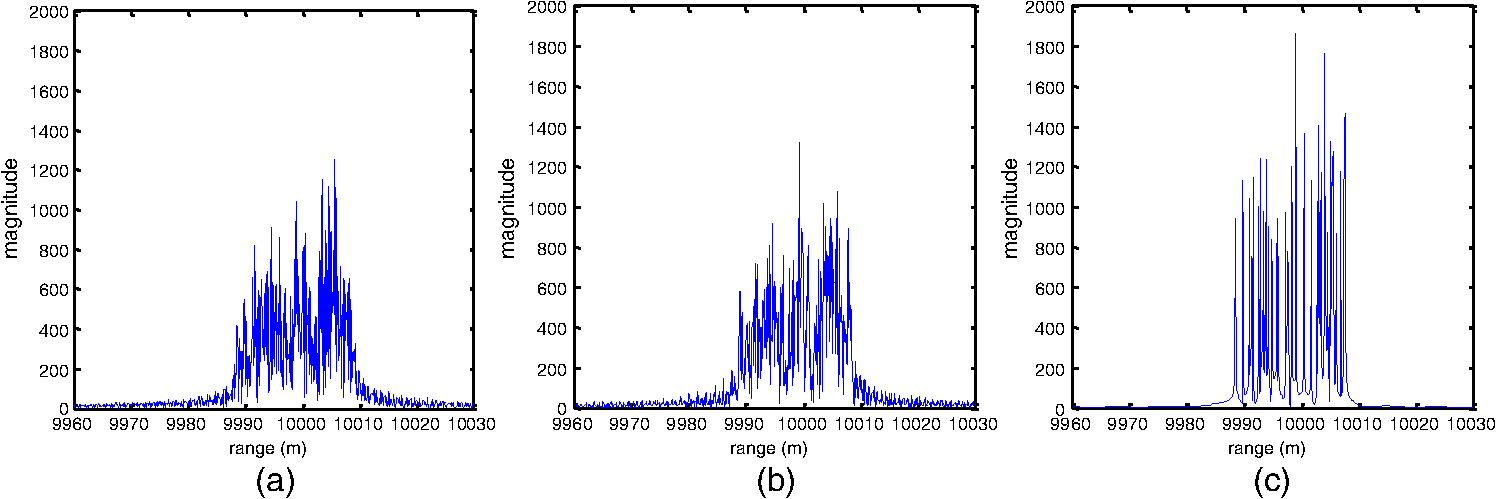 Fig. 9The imaging results (a) without motion compensation and (b) with motion compensation using CCIFM, and (c) with motion compensation using MCCM. 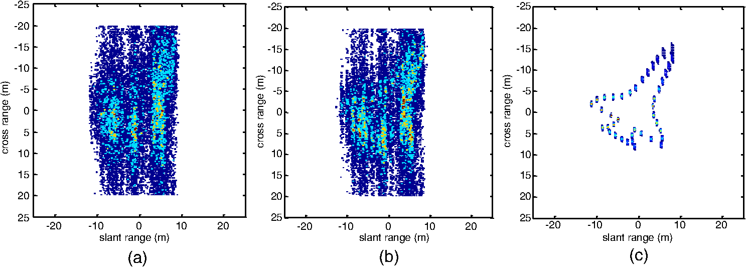 Table 1Simulation parameters.
Figure 8(a) presents the synthesized range profile without motion compensation, from which one can see that the high-speed motion-induced phase errors make the range profile seriously smear. Figure 8(b) shows the result with motion compensation conducted using CCIFM. Because CCIFM cannot correctly measure the velocity of the MSC target, Fig. 8(b) scarcely improves compared to Fig. 8(a). Figure 8(c) gives the synthesized range profile with motion compensation conducted using SCS-MCCM; it is very well profiled as we expected. Figure 9(a) shows the 2-D imaging result without motion compensation. Due to the high speed of the target, the motion-induced phase errors make the image seriously blurred. Figures 9(b) and 9(c) are the images with motion compensation conducted using CCIFM and SCS-MCCM, respectively. As before, one can see that CCIFM does not work in the MSC target case. However, SCS-MCCM can handle this case and the radar image is very well focused, as shown in Fig. 9(c). The results of Fig. 9 also indicate that the high-speed motion-induced errors affect not only the range profiles, but also azimuth focusing. The above simulation experiments demonstrate that the proposed velocity measurement method for a high-speed target based on SCS is valid and effective, and the resulting measurement error can meet the requirement for high-resolution imaging. Figures 10 and 11 present the real velocity measurement results using the same parameters and geometry as in the previous imaging simulation. The solid curves represent the estimated values versus the used number of received pulses. The dotted lines represent the real velocity set in the simulation, which is . From these two figures, one can see that the curves fluctuate severely and the measurement errors are quite large for both SSC and MSC targets when only several pulses are received and used. With an increase in the number of received pulses, the fluctuations of the curves quickly reduce, and the estimated values gradually approach the true value. The variance of the curve in Fig. 11 is larger than that in Fig. 10 because the velocity measurement accuracy for the SSC target is better than that for the MSC target. If we just take into account the parts of curves with a pulse number , we get the mean values of in Fig. 10 and in Fig. 11, respectively, i.e., the relative measurement errors are and 2.1%, respectively. 6.ConclusionHigh-resolution radar imaging of a high-speed target using SCS must properly solve the problem of motion estimation and compensation. We propose the SCS-MCCM to accurately measure the velocity of a high-speed target with MSCs, which is the first step for high-resolution imaging. Detailed analysis and derivations of the proposed method are presented. Although it is not the most accurate method of velocity measurement with SCS, the advantages of SCS-MCCM make it practically applicable and easy to adopt. It can measure the target radial velocity by using only the echoes of subpulses within a burst, so it does not require a high repetition frequency of burst and, thus, has a large unambiguous measurement range. If the target moves straight, this method can also be used to measure the real velocity of the target. To show the validation and effectiveness of the method, simulations for an MSC target are conducted, which clearly show that the radar image is very well focused after performing motion compensation using the proposed method, but is not focused by using CCIFM; at the same time, the real target velocity is also well estimated. We should emphasize that there is still a room for improving the velocity measurement accuracy for an MSC target with the proposed method, and this is our next effort. ReferencesD. R. Wehner, High-Resolution Radar, 2nd ed.Artech House, Boston/London
(1995). Google Scholar
N. Levanon,
“Stepped-frequency pulse-train radar signal,”
IEE Proc. Radar, Sonar Navig., 149
(6), 297
–309
(2002). http://dx.doi.org/10.1049/ip-rsn:20020432 IRSNE2 1350-2395 Google Scholar
Q. ZhangY.-Q. Jin,
“Aspects of radar imaging using frequency-stepped chirp signals,”
EURASIP J. Appl. Signal Process., 2006 1
–8
(2006). http://dx.doi.org/10.1155/ASP/2006/85823 1110-8657 Google Scholar
N. LevanonE. Mozeson, Radar Signals, John Wiley & Sons, Hoboken, New Jersey
(2003). Google Scholar
J. S. Son, Range-Doppler Radar Imaging and Motion Compensation, Artech House, Boston/London
(2000). Google Scholar
T. LongL. Ren,
“HPRF pulse Doppler stepped frequency radar,”
Sci. China, 52
(5), 883
–893
(2009). http://dx.doi.org/10.1007/s11432-009-0087-8 1009-2757 Google Scholar
B. D. RiglingG. S. Goley,
“On the feasibility of ISAR processing of stepped frequency waveforms,”
in 2013 IEEE Radar Conf.,
1
–6
(2013). Google Scholar
T. J. AbatzoglouG. O. Gheen,
“Range radical velocity and acceleration MLE using radar LFM pulse train,”
IEEE Trans. Aerosp. Electron Syst., 34
(4), 1
–4
(1998). http://dx.doi.org/10.1109/7.722676 IEARAX 0018-9251 Google Scholar
Y. Liuet al.,
“Motion compensation of moving targets for high range resolution stepped-frequency radar,”
Sensors, 8
(5), 3429
–3437
(2008). http://dx.doi.org/10.3390/s8053429 SNSRES 0746-9462 Google Scholar
P. FrancescoT. Enrico,
“Motion compensation for a frequency stepped radar,”
in Proc. of Waveform Diversity and Design Conf.,
255
–259
(2007). Google Scholar
B. LiuW. Chang,
“Range alignment and motion compensation for missile-borne frequency stepped chirp radar,”
Prog. Electromagn. Res., 136 523
–542
(2013). http://dx.doi.org/10.2528/PIER12110809 PELREX 1043-626X Google Scholar
F. BerizziM. Martorella,
“A Capria. A contrast-based algorithm for synthetic range-profile motion compensation,”
IEEE Trans. Geosci. Remote Sens., 46
(10), 3053
–3061
(2008). http://dx.doi.org/10.1109/TGRS.2008.2002576 IGRSD2 0196-2892 Google Scholar
S. HuixiaL. Zheng,
“Compound velocity measurement based on modulated frequency stepped radar,”
Syst. Eng. Electron., 33
(3), 539
–543
(2011). 1004-4132 Google Scholar
H. YuanS. WenZ. Cheng,
“Simultaneous radar imaging and velocity measuring with step frequency waveforms,”
J. Syst. Eng. Electron., 20
(4), 741
–747
(2009). 1004-4132 Google Scholar
W. FeiL. Teng,
“A new method of velocity estimation for inverse V-shape stepped frequency signal,”
in CIE'06 Int. Conf. on Radar,
1
–3
(2006). Google Scholar
G. Liet al.,
“Range and velocity estimation of moving targets using multiple stepped-frequency pulse trains,”
Sensors, 8
(2), 1343
–1350
(2008). http://dx.doi.org/10.3390/s8021343 SNSRES 0746-9462 Google Scholar
B. Yun-xiaet al.,
“Velocity measurement and compensation method based on range profile cross-correlation in stepped-frequency radar,”
Syst. Eng. Electron., 30
(11), 2112
–2115
(2008). 1004-4132 Google Scholar
L. Zhaoet al.,
“A novel method of ISAR imaging for high speed targets using stepped-frequency chirp waveform,”
in 2011 IEEE CIE Int. Conf. on Radar,
1604
–1607
(2011). Google Scholar
G. F. XiaH. Y. SuP. K. Huang,
“Velocity compensation methods for a LPRF modulated frequency stepped frequency (MFSF) radar,”
J. Syst. Eng. Electron., 21
(5), 746
–751
(2010). http://dx.doi.org/10.3969/j.issn.1004-4132.2010.05.005 Google Scholar
Z. YunhuaW. JieL. Haibin,
“Two simple and efficient approaches for compressing stepped chirp signals,”
in 2005 Asia-Pacific Microwave Conf.,
690
–693
(2005). Google Scholar
BiographyWenshuai Zhai is an assistant professor with the Key Laboratory of Microwave Remote Sensing, Center for Space Science and Applied Research, Chinese Academy of Sciences. She received her BS degree in electronic engineering from Zhejiang University in 2004, and her MS and PhD degrees in electromagnetic field and microwave technology in 2007 and 2013, respectively. Her current research interests include SAR/ISAR imaging and high-resolution radar signal processing. Yunhua Zhang is a professor with the Key Laboratory of Microwave Remote Sensing, Center for Space Science and Applied Research, Chinese Academy of Sciences. He received his BS degree from Xidian University, Xi’an, and his MS and PhD degrees from Zhejiang University, Hangzhou, China, in 1989, 1993, and 1995, respectively, all in electrical engineering. His research interests cover the system design and signal processing of microwave sensors and high-resolution radar, as well as computational electromagnetics. |