Comparison of satellite chlorophyll a algorithms for the Baltic Sea

Monika Woźniak; Katarzyna M. Bradtke; Adam Krężel

doi:10.1117/1.JRS.8.083605

30 June 2014 Comparison of satellite chlorophyll a algorithms for the Baltic Sea

Monika Woźniak, Katarzyna M. Bradtke, Adam Krężel

Author Affiliations +

Journal of Applied Remote Sensing, Vol. 8, Issue 1, 083605 (June 2014). https://doi.org/10.1117/1.JRS.8.083605

Abstract

Chlorophyll a (chl-a) products calculated using medium resolution imaging spectrometer (MERIS) data were tested. The satellite products were compared to chl-a concentrations measured in surface waters between 2003 and 2011 throughout the Baltic Sea. Image processing was performed with two neural-network-based MERIS data processors: the Case-2 Water Properties processor developed at the Freie Universität Berlin (FUB) and the Case-2 Regional processor of the German Institute for Coastal Research (C2R). Additionally, two algorithms for deriving chl-a concentrations from atmospherically corrected reflectances originally designed for Moderate Resolution Imaging Spectroradiometer and Sea-viewing Wide Field-of-view Sensor radiometers and adapted to Baltic Sea conditions were tested (algorithms denoted further as MD and SW respectively). The effectiveness of the Improved Contrast between Ocean and Land (ICOL) processor was also verified. Our results showed that the accuracy of chl-a concentration retrieval from satellite data varies depending on the location of the area. The difference in the statistical error between results from optically different coastal and open sea waters was as high as 200%. The most accurate results for the coastal zone were noted for the standard chl-a FUB processor product, while in open sea waters the highest accuracy was noted for the MD and SW algorithms with reflectance derived from the FUB processor.

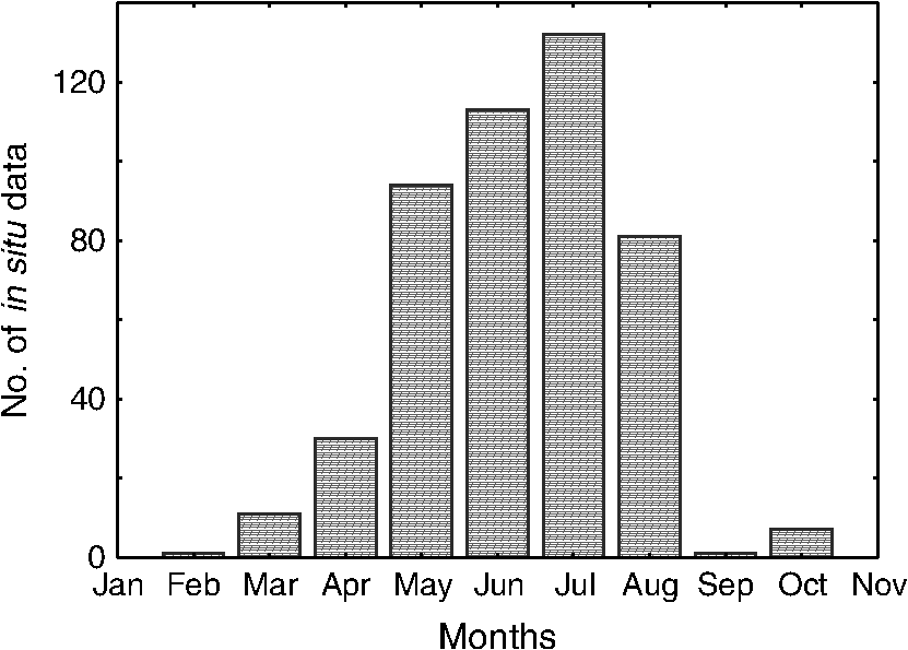
1. Introduction

Phytoplankton is an important component of all marine ecosystems. Chlorophyll $a$ (chl- $a$ ) is the most common photosynthetically active pigment present in all phytoplankton species. Its concentration is a good indicator of phytoplankton biomass and it is frequently used for water quality assessment.¹ The concentration of this pigment is influenced by environmental factors such as water temperature, light intensity, and nutrient concentrations.²^,³The presence of chlorophyll $a$ influences the optical properties of sea water; therefore, concentrations of it can be retrieved from data acquired by satellite spectrometers operating in the solar reflective spectral range. These data can be used to monitor spatial and seasonal variations in the near-surface phytoplankton biomass. Estimations of concentrations of optically active sea water components are based on their absorption and scattering properties,⁴ and there are numerous algorithms to calculate chl- $a$ using satellite remote sensing techniques. These algorithms work satisfactorily with Case-1 waters,⁵^,⁶ but with more complex Case-2 waters their accuracy is not as good because the radiance signal recorded by satellite sensors is influenced by high concentrations of colored dissolved organic matter (CDOM, also called yellow substances) and suspended particulate matter (SPM) in which detritus and mineral particles can occur in varying proportions.⁷^–⁹

The Baltic Sea, which is a Case-2 water reservoir, is one of the largest, semi-enclosed, brackish seas in the world. Its freshwater content is strongly linked to nutrient inputs from its densely populated, intensively cultivated catchment areas, and the atmosphere.¹ Excess nutrient input is one of the major causes of eutrophication in the Baltic Sea, and it results in frequent algal blooms that frequently cover major parts of the sea.¹⁰^,¹¹ Some bloom-forming organisms, such as cyanobacteria, can form extensive summer blooms that can be toxic to other organisms, including humans. They can also affect the recreational use of coastal areas. Therefore, it is essential to predict and monitor the development of phytoplankton blooms and to study them with relevant spatial and temporal resolutions. Remote sensing techniques can provide the extensive spatial and temporal coverage required to study this problem; however, standard remote sensing algorithms developed for Case-2 waters often fail in the complex, CDOM-rich waters of the Baltic Sea.

Satellite algorithms for chl- $a$ concentration retrieval in the Baltic Sea region have been developed over the course of many projects.¹²^,¹³ The algorithms for calculating concentrations of optically active sea water components, including chl- $a$ concentrations, apply to the visible (VIS) part of the electromagnetic spectrum measured by satellite sensors such as the Sea-viewing Wide Field-of-view Sensor (SeaWIFS), the Moderate Resolution Imaging Spectroradiometer (MODIS), and the medium resolution imaging spectrometer (MERIS). There are also plans to launch a new European Space Agency (ESA) satellite—the Sentinel-3, which will carry the Ocean and Land Colour Instrument (OLCI) radiometer.

The aim of this work was to compare the performance of standard chl- $a$ concentration products of two different neural-network-based (NN) processors developed for MERIS data and two other band ratio algorithms for retrieving chl- $a$ concentrations acquired for the Baltic Sea. The processors considered, the Case-2 Water Properties processor developed at the Freie Universität Berlin (FUB) and the Case-2 Regional (C2R) processor of the German Institute for Coastal Research (C2R), are recommended for Case-2 waters.¹⁴^–¹⁷ The band ratio algorithms, developed during the DESAMBEM project (DESAMBEM—Development of a Satellite Method for Baltic Ecosystem Monitoring for creating mathematical models and a complex algorithm for the remote sensing of the Baltic ecosystem and its primary production.), were proposed by Woźniak et al.¹⁸ and were tested by Darecki et al.¹⁹ All chl- $a$ products were tested with and without Improved Contrast between Ocean and Land (ICOL) processing.

The processors mentioned above are based on NNs, but the C2R processor algorithms apply to waters producing radiance reflectances within eight spectral bands, whereas FUB uses independent NN for each component and estimates concentrations directly from collected radiances at the top of the atmosphere (TOA). These have already been tested in various Baltic Sea regions: in the northwest,¹³^,²⁰ Skagerrak,²¹ open sea areas,²² and in the southeast Baltic Sea.¹ All these investigations proved the utility of satellite remote sensing for surface water environmental monitoring. However, the datasets used in the previous validation processes of MERIS products were usually small and concentrated in particular regions of the Baltic Sea. In the current project, we focused on the chl- $a$ concentration products retrieved from MERIS data for the whole area of the Baltic Sea. Even though the Envisat satellite carrying the MERIS sensor is no longer operational, the data from this sensor are still useful because of the very large historical database. Moreover, the Sentinel-3 OLCI radiometer will include all spectral bands of the MERIS radiometer. Therefore, the assessment of the algorithms presented in this study can still be useful.

2. Materials and Methods

2.1.

Study Area

In our work, the area of interest was divided into two subareas—coastal and open sea waters. The coastal area was designated as the area up to 10 km from the shore. This distance is specified in MERIS protocols to avoid the effects of coastal aerosol influence.²³ Optical properties of coastal waters are much more complex and vary from those in the open sea because of the influence of land and river plumes. Moreover, the coastal zone is often affected by upwelling, which causes transparent near-bottom and turbid surface waters to mix.

The optical parameters that characterize Baltic Sea waters are highly variable spatially and temporally. According to HELCOM reports,²⁴ the mean chl- $a$ concentration is about $2.9 mg / m^{3}$ during spring, $2.3 mg / m^{3}$ in summer, and $2.2 mg / m^{3}$ in winter. The highest concentration observed during a spring bloom was $27 mg / m^{3}$ . Much higher values are expected in summer during the dense surface accumulation of bloom-forming organisms. The concentration of chl- $a$ during a summer phytoplankton bloom can reach as much as $120 mg / m^{3}$ .²⁵ The formation of phytoplankton blooms in the Baltic Sea follows similar patterns every year. Diatoms and dinoflagellates dominate in spring and fall, whereas cyanobacteria usually form the summer blooms. The first spring algal blooms are usually observed at the end of April in the southwest Baltic Sea. From July until early fall, when the ratio of dissolved inorganic nitrogen to phosphorus (DIN:DIP) is low, blooms in the open Baltic Sea are formed mostly by nitrogen-fixing cyanobacteria like Nodularia spumigena and Aphanizomenon flos-aquae. The area of these blooms can cover up to 15% of the total area of the Baltic Sea.²⁶ All phytoplankton groups contain chlorophyll $a$ along with other accessory pigments in their cells.

The optical properties of Baltic Sea waters are mainly influenced by CDOM, which occurs in very high concentrations in comparison to those in other seas. According to Kowalczuk,²⁷ the yellow substance absorption coefficient of $λ = 400 nm$ , $a_{CDOM} (400)$ varies from 0.23 to 1.84 $1 / m$ for the open sea and from 0.26 to 2.39 $1 / m$ for the coastal waters. The highest values of $a_{CDOM} (400)$ are observed in spring and are caused by the largest input of river waters. The slope coefficient of the yellow substance absorption spectrum ranges between 0.004 and 0.032 for the open sea and between 0.007 and 0.031 for the coastal waters, and it does not exhibit any seasonal variability. Moreover, the concentration of SPM influences the optical properties of the sea water. According to Wozniak et al.,²⁸ SPM concentrations vary between 0.36 and $15.7 g / m^{3}$ with a mean value of $2.42 g / m^{3}$ .

2.2.

In Situ Data

In situ chl- $a$ concentration data were obtained from the International Council for the Exploration of the Sea (ICES) Oceanographic Database and Services,²⁹ which is recommended by, among others, the International Ocean-Colour Coordinating Group (IOCCG).³⁰ The service mainly contains Baltic Sea Monitoring (HELCOM) data. However, data provided by other institutions are also available in this database. For the purpose of this study, we chose chl- $a$ concentrations measured in surface waters no deeper than 2 m. The sampling points covered the entire area of the Baltic Sea (Fig. 1), and all the algorithms tested in this study were validated using the same dataset. It has to be mentioned that we had no information on the techniques used in the chl- $a$ concentration measurements. Therefore, we assumed that high-performance liquid chromatography (HPLC), spectrophotometric, or fluoromethric methods could have been used. According to some publications,¹²^,³¹ there is a difference in the magnitude of chl- $a$ concentrations obtained using different techniques. For example, it has been reported¹² that the HPLC method always produces lower chl- $a$ concentrations (by a factor of 0.64) than the spectrophotometric method regardless of the chl- $a$ concentrations in the samples. This was explained by the influence of pheopigments on the result of measurements performed using the spectrophotometric method, although our analysis of the samples taken in the Gulf of Gdansk show a much smaller difference between the concentration of chl- $a$ obtained with both methods (regression: $chl - a_{HPLC} = 0.98 {chl - a_{spec}} - 0.09$ , $R^{2} = 0.89$ ). However, taking into consideration the uncertainty about the method, we did not draw any conclusions about the real accuracy of any of the algorithms, but only compared them. Each one was tested on the same database, so differences in techniques used in the chl- $a$ concentration measurements should not influence our conclusions. Because of the patchiness effect and the strong dynamics of the water,³² comparisons among in situ data (from one point) and satellite data (average from an area measuring $1.2 \times 1.2 km$ ) always produces some errors which exceed the errors arising from the using of different in situ measurement methods. Moreover, the time shift of satellite overpass and in situ sampling that can be as much as a few hours and differences in typical optical properties between coastal and open sea waters are also sources of errors in calculated chl- $a$ concentration values. These errors are much higher than those that arise when using different in situ measurement methods. The validation data were chosen for days when MERIS data were available (Fig. 2); however, sampling times were not accounted for. MERIS overpasses over the Baltic Sea were between 09:00 and 11:00, whereas $> 50 %$ of the in situ data were gathered between 06:00 and 14:00. The majority of the data considered were collected in spring and summer because the Baltic Sea is frequently overcast during fall and winter (Fig. 3). However, the in situ concentration values ranged between $< 1$ and about $35 mg / m^{3}$ (Table 1), which reflects a wide range of situations observed in other seasons as well. Moreover, all the in situ measurement points considered were located at least 1 km from the coastline to avoid using pixels partly covered by land in the comparison.

Fig. 1

Spatial distribution of in situ data (chlorophyll $a$ concentration measurement stations in the Baltic Sea) used for the satellite algorithm evaluation.

Fig. 2

Diurnal distribution of the in situ data used for satellite algorithm evaluation.

Fig. 3

Seasonal distribution of the in situ data used for satellite algorithm evaluation.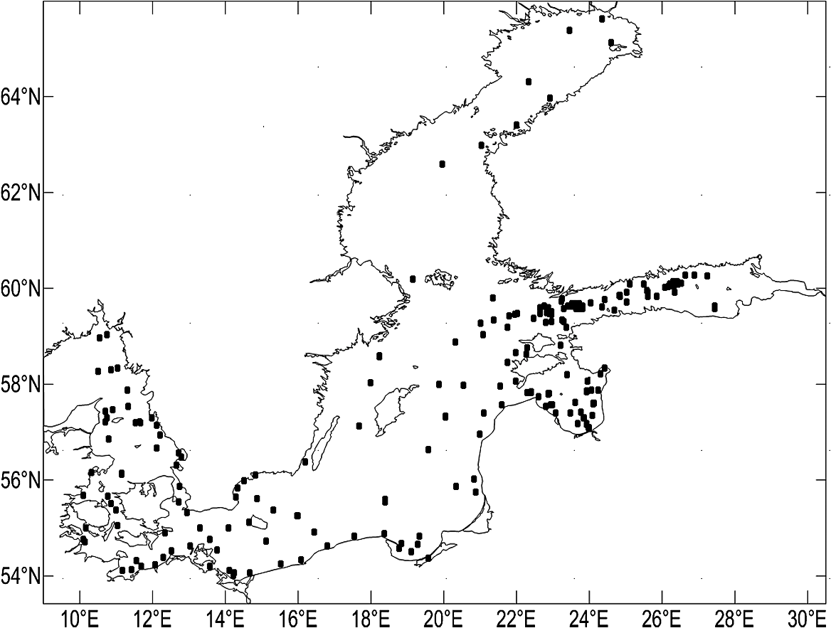

Table 1

Descriptive statistics of in situ concentrations of chlorophyll a taken for satellite algorithm evaluations.

$No . of data = 470$	Mean	Median	Minimum	Maximum	Standard Deviation	Lower Quartile	Upper Quartile
in situ [ $mg / m^{3}$ ]	3.73	2.50	0.17	33.20	3.79	1.26	4.90

2.3.

Satellite Data Acquisition and Processing

The MERIS was mounted on the Envisat satellite platform and launched by the ESA in 2002. The MERIS sensor worked within the VIS and near-infrared (NIR) spectral range (400 to 900 nm) with a wavelength configuration sensitive to the most important optically active water constituents. MERIS acquired data in 15 spectral bands. For the purpose of this study, Level 1b reduced resolution (RR) data from the period between 2003 and 2011 were downloaded from the MERCI server developed by Brockmann Consult under contract to the ESA.³³ The resolution of the RR data is 1.2 km. Cloudiness assessment was performed by visually evaluating RGB images. We accounted only for pixels that were not covered by clouds. Conclusively, 470 pairs of chlorophyll $a$ concentrations (derived from satellite data and in situ measurements) were chosen the entire period of the Envisat mission, i.e., from 2003 to 2011. Figure 4 presents the data processing sequence. In the first step, the radiometric correction including the “smile effect” correction, and equalization was performed. The “smile effect” correction is performed in order to correct the MERIS reflectance for the small scale due to the nonconstant central wavelength of a given band across the field–of-view.³⁴ Equalization removes detector-to-detector systematic radiometric differences and results in the diminution of the vertical stripping observed on L1b products.³⁵ Level 1c data contain signals from the TOA at satellite level. TOA radiance is influenced both by the light attenuation processes occurring in the Earth’s atmosphere between the sea surface and the radiometer and some additional radiation coming from the atmosphere (atmospheric path radiance). Only a small part (0% to 30% depending on the wavelengths and environmental conditions) of signals measured within the VIS and NIR range of the electromagnetic spectrum that reach satellite sensors comes from the water. This information has to be retrieved in order to monitor water surfaces. Therefore, L1c data were recalculated into reflectances at sea level (atmospherically corrected). A suitable atmospheric correction is crucial for obtaining accurate values of water-leaving reflectance.¹³ In this project, the data were processed using two different processors recommended for Case-2 waters for MERIS data: C2R and FUB. These algorithms are plugged into the BEAM software¹⁵^,¹⁶ used for data processing. Both processors include algorithms for atmospheric corrections and for deriving Level 2 water quality parameters, which are calculated directly using L1c data. In our study, we generated two standard products of chlorophyll $a$ concentration named ST_C2R and ST_FUB. Moreover, atmospherically corrected reflectances were used to retrieve chlorophyll $a$ concentrations by using two band ratio algorithms originally derived for MODIS (MD) and SeaWiFS (SW) radiometers and adapted to local conditions within the framework of the DESAMBEM project.¹⁸ Thus, the following four chlorophyll $a$ products were generated: MD_C2R and SW_C2R using reflectances produced by the C2R processor, and MD_FUB and SW_FUB using reflectances obtained using FUB. The same procedure was repeated using the L1N product (after ICOL correction) instead of L1c (without ICOL correction) as input data for the C2R and FUB processors. The L1N data are generated by applying the ICOL processor to L1c data in order to correct the adjacency effect. To indicate differences, the names of the products obtained with ICOL were preceded by “ICOL” (ICOL_ST_C2R, ICOL_MD_C2R, ICOL_SW_C2R, ICOL_ST_FUB, ICOL_MD_FUB, ICOL_SW_FUB). For the final step, all data were reprojected with Lambert azimuthal equal area projection.

Fig. 4

Sequence of the satellite data processing steps (abbreviations explained in Sec. 2.3).

2.3.1.

Standard Chlorophyll a Products

The C2R of the German Institute for Coastal Research derives Level 2 water quality parameters of coastal waters from MERIS Level 1b data. C2R uses NN procedures to retrieve water-leaving reflectance from calculated TOA reflectance after ozone, water vapor, and surface pressure corrections in eight MERIS bands. These reflectances, which are the output of the atmospheric correction, are then input in to the algorithms of the Regional Bio-Optical Model. The algorithms derive data of inherent optical properties, total scattering of particles, absorption coefficients of phytoplankton pigments, and the absorption of dissolved organic matter—all at 443 nm. These IOPs are used to determine chlorophyll $a$ concentrations.¹⁷

The Case-2 Water Properties processor, developed at the FUB, is based on four separate artificial NNs that were trained using results of extensive radiative transfer simulations with MOMO code by taking into account varying atmospheric and oceanic conditions. One network performs atmospheric corrections and derives water-leaving reflectance at eight spectral bands, including aerosol optical depths at four spectral bands, while the other three networks retrieve the concentrations of water constituents, including chlorophyll $a$ , directly from the TOA measured radiances.¹⁵^,³⁶

2.3.2.

Regional chl-a Algorithms

Two tested band ratio algorithms for retrieving chl- $a$ concentration acquired for the Baltic Sea (MD and SW) were developed during the DESAMBEM project¹⁸ [Eqs. (1) and (3)]

• SeaWiFS algorithm (SW):
Eq. (1)
$C_{a} {(0) = 10}^{(1.311 - 0.7875 X R - {0.4935 X R}^{2})},$
where
Eq. (2)
$X R = \frac{R_{rs} (510 nm) - R_{rs} (665 nm)}{R_{rs} (555 nm) - R {}_{rs} (665 nm)}$
• MODIS algorithm (MD):
Eq. (3)
$C_{a} (0) = 10^{(1.102 - 0.8708 X R - {0.3449 X R}^{2})},$
where
Eq. (4)
$X R = \frac{R_{rs} (490 nm) - R_{rs} (665 nm)}{R_{rs} (550 nm) - R {}_{rs} (665 nm)},$
Where $C_{a} (0) (mg / m^{3})$ is the surface layer concentration of chlorophyll $a$ and $R_{rs} (λ) (1 / sr)$ is the remote sensing reflectance at a wavelength $λ$ .

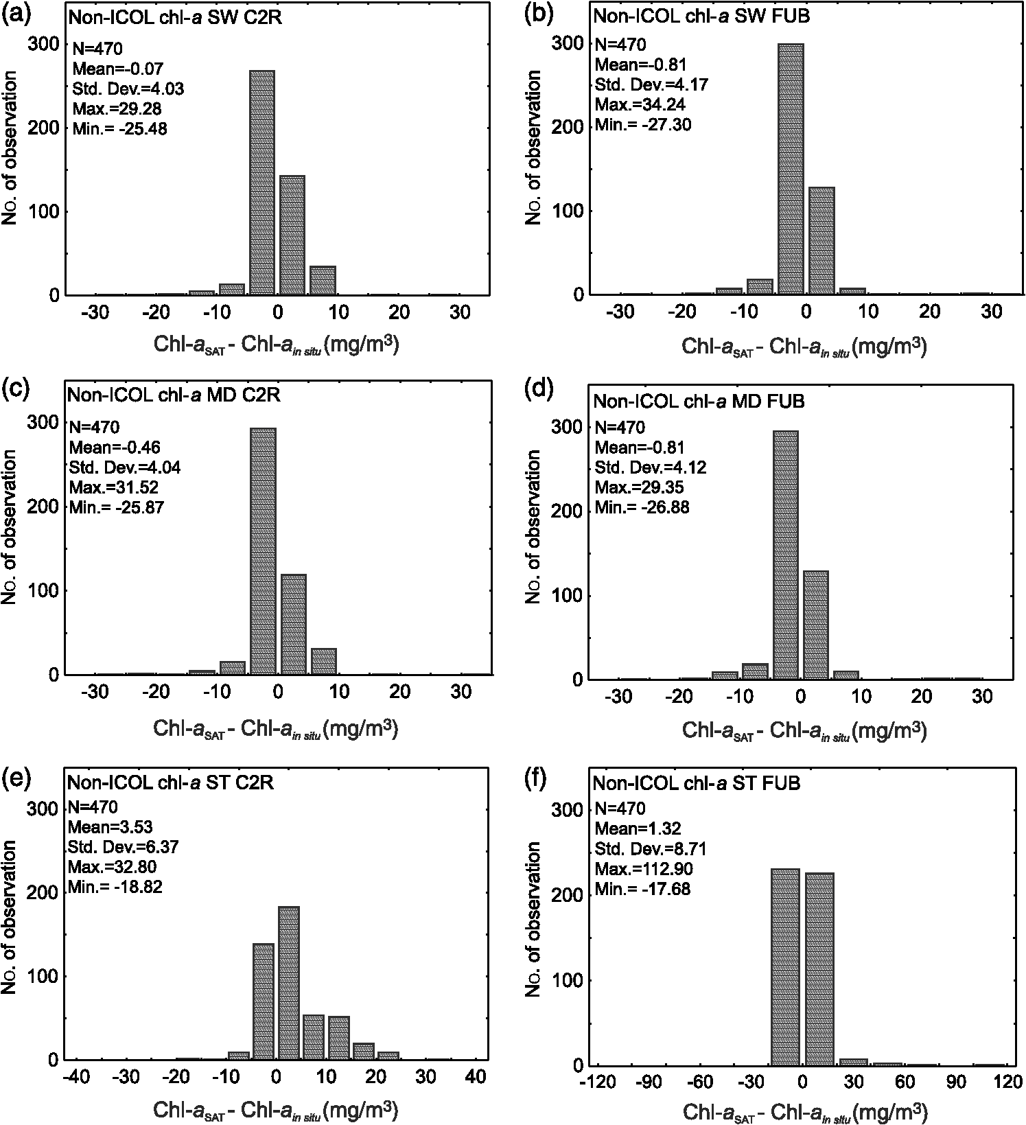
The coefficients were calibrated using a large set of Baltic Sea measurement data. The spectral bands applied corresponded to the MERIS spectral bands. The assessment of nine different algorithms for chl- $a$ concentration and other optically active components for the Baltic Sea were proposed by Woźniak et al.³⁷ at the International Ocean Colour Science Meeting, and they confirmed that the algorithms proposed in the DESAMBEM project have the lowest bias; thus, they were chosen for this project. Reflectances retrieved with either the C2R or FUB processors were taken as the input data in our work with the preceding algorithms.

2.4.

Statistical Analysis

The dataset for the statistical analysis was created by extracting the values of the MERIS-derived concentrations from pixels located at the position of sampling points of the in situ data. Only cloud-free pixels were analyzed, and arithmetic statistics were used to evaluate our results. We applied this approach in order to compare our results to other published data referring to the Baltic Sea region.¹^,¹²^,¹⁸ The differences between satellite and in situ chl- $a$ concentrations are not symmetrically distributed. Therefore, the errors were quantified using relative metrics: the relative mean error (systematic error) [Eq. (5)], which is also called mean normalized bias (MNB), as well as the standard deviation (statistical error) [Eq. (6)]. All errors were calculated for products derived both from L1c (without ICOL) and L1N (with ICOL) processing

Eq. (5)

〈 ε 〉 = \frac{1}{N} \sum_{i = 1}^{N} (ε_{i}) \times 100 %,

Eq. (6)

σ_{ε} = \sqrt{\frac{1}{N} \sum_{i = 1}^{N} {(ε_{i} - 〈 ε 〉)}^{2}} \times 100 %,

where

ε_{i} = \frac{x_{i, MERIS} - x_{i, i n s i t u}}{x_{i, i n s i t u}},

where

x_{i, MERIS}

is a calculated value with the use of MERIS data and

x_{i, i n s i t u}

is a measured value.

3. Results

3.1.

Comparison of chl-a Products Without ICOL Correction

The range of the in situ concentrations (Table 1) remained in good agreement with the results of all the algorithms tested, except for the standard product of chlorophyll $a$ concentration calculated with the FUB processor (ST_FUB). In this case, the maximum value was about four times higher ( $118.40 mg / m^{3}$ ) than the maximum value in the reference dataset ( $33.20 mg / m^{3}$ ) (Table 2). However, the best fit of the median and the upper and lower quartiles of in situ to satellite-derived data was observed for FUB processor products MD ( $median = 1.60 mg {/ m}^{3}$ , $lower quartile = 0.54 mg / m^{3}$ , and $upper quartile = 4.02 mg / m^{3}$ ) and SW ( $median = 1.71 mg / m^{3}$ , $lower quartile = 0.73 mg / m^{3}$ , and $upper quartile = 3.82 mg / m^{3}$ ) (Table 2). Decreases in relative statistical error were observed with increasing concentrations of chl- $a$ (Table 3). The highest error was noted for concentrations lower than $1 mg / m^{3}$ (from 254% for ST_FUB to as high as 966% for ST_C2R). The dispersion of the differences between calculated and measured data on histograms (Fig. 5) was the smallest for the SW_C2R (between $- 25.48$ and $29.28 mg / m^{3}$ with a mean value of $- 0.07 mg / m^{3}$ ), whereas the highest was for the ST_FUB (between $- 17.68$ and $112.90 mg / m^{3}$ with a mean value of $1.32 mg / m^{3}$ ) algorithm.

Table 2

Descriptive statistics of chlorophyll a concentrations derived from satellite data (chl-aSAT without ICOL correction, using both processors—C2R and FUB, and all algorithms tested (ST, MD, SW).

$No . of data = 470$	Mean	Median	Minimum	Maximum	Standard Deviation	Lower Quartile	Upper Quartile
ST C2R [ $mg / m^{3}$ ]	7.72	4.68	0.22	36.17	7.37	1.34	11.04
MD C2R [ $mg / m^{3}$ ]	3.49	2.08	$< 0.01$	44.71	4.04	0.20	5.31
SW C2R [ $mg / m^{3}$ ]	3.89	2.52	0.01	42.02	4.04	0.54	5.66
MD FUB [ $mg / m^{3}$ ]	3.17	1.60	$< 0.01$	33.65	4.11	0.54	4.02
SW FUB [ $mg / m^{3}$ ]	3.18	1.71	$< 0.01$	33.59	4.08	0.73	3.82
ST FUB [ $mg / m^{3}$ ]	4.94	2.46	0.16	118.40	9.60	1.24	5.62

Table 3

Systematic (〈ε〉) and statistical errors (σε) of chlorophyll a concentrations derived from satellite data without ICOL correction, using both processors—C2R and FUB, and all algorithms tested (ST, MD, SW), calculated for different ranges of chl-a concentrations.

	chl- $a$ (0-1) [ $mg / m^{3}$ ]		ch- $a$ (1-5) [ $mg / m^{3}$ ]		chl- $a$ (5-10) [ $mg / m^{3}$ ]		chl- $a > 10$ [ $mg / m^{3}$ ]
	$〈 ε 〉$ [%]	$σ_{ε}$ [%]	$〈 ε 〉$ [%]	$σ_{ε}$ [%]	$〈 ε 〉$ [%]	$σ_{ε}$ [%]	$〈 ε 〉$ [%]	$〈 ε 〉$ [%]
ST C2R	503	966	149	260	77	113	14	71
MD C2R	121	455	4	124	18	52	$- 34$	79
SW C2R	174	484	22	129	$- 11$	53	$- 32$	75
MD FUB	130	635	$- 15$	105	$- 12$	81	$- 59$	31
SW FUB	150	714	$- 12$	107	$- 16$	80	$- 57$	30
ST FUB	152	254	24	127	74	287	$- 11$	73

Fig. 5

Distribution of the differences between chlorophyll $a$ concentration measured in situ (chl- $a_{i n s i t u}$ ) and derived from satellite data (chl- $a_{SAT}$ ) without ICOL correction, using both processors: C2R (a, c, and e) and FUB (b, d, and f), and all tested algorithms (ST, MD, and SW) described in the text.

3.2.

Benefits of ICOL Correction

First, we checked the influence of using ICOL correction without accounting for sampling point locations. The results showed significant improvement, by about 100%, only for the band ratio algorithms applied for the FUB derived reflectances. Statistical errors $σ_{ε}$ were reduced from 265% to 181% for the MD algorithm and from 294% to 187% for the SW algorithm after ICOL correction (Table 4). No improvement was noted in the other cases. Standard chl- $a$ concentration products obtained using FUB and C2R processors (ST_FUB and ST_C2R) were not significantly changed by ICOL ( $σ_{ε}$ was 193% and 448% before ICOL correction and 194% and 463% after, respectively). However, the results of band ratio algorithms applied for C2R-derived reflectances were slightly worse after using ICOL correction ( $σ_{ε}$ was 206% for the MD algorithm and 221% for the SW algorithm before ICOL correction and 221% and 235% after, respectively) (Table 4). The application of this processor is not always advisable because of the lengthy computation time of at least a half-an-hour for one RR image of the Baltic Sea. The statistics of dispersion on the histograms of the differences between the MERIS and in situ data after the ICOL processor changed only slightly (Fig. 6). The smallest dispersion was noted for SW_C2R (between $- 20.59$ and 15.71 with a mean value of 0.16), whereas the highest was for the ST_FUB algorithm (between $- 17.67$ and 112.90 with a mean value of 1.22). Data scattering was greater when the ICOL processor was not applied for ST_FUB ( $R 2 = 0.32$ before and $R 2 = 0.48$ after ICOL correction) (Fig. 7), whereas the coefficient of determination for both SW_FUB and MD_FUB was smaller after ICOL correction. Nevertheless, improvements in the statistical error of these two algorithms was significant (Table 4). Although the statistics for the band ratio algorithms (MD and SW) were the best, these algorithms significantly underestimated the concentrations corresponding to in situ values lower than ${5 mg / m}^{3}$ (Fig. 7). When all the data were considered together, the best results were obtained using the band ratio algorithms with the FUB processor after ICOL correction (ICOL_MD_FUB and ICOL_SW_FUB) (Table 4). The results are not surprising, because, according to Kratzer,¹³ the ICOL processor should improve the level 2 data.

Table 4

Comparison of systematic (〈ε〉) and statistical errors (σε) of chlorophyll a concentrations derived from satellite data for all the algorithms tested (ST, MD, SW) obtained with and without ICOL corrections.

Arithmetic statistics for all stations $No . of data = 470$
	NON-ICOL		ICOL
	$〈 ε 〉$ [%]	$σ_{ε}$ [%]	$〈 ε 〉$ [%]	$σ_{ε}$ [%]
ST C2R	181	448	178	463
MD C2R	15	206	13	221
SW C2R	35	221	35	235
MD FUB	5	265	13	181
SW FUB	9	294	16	187
ST FUB	51	193	45	194

Fig. 6

Distribution of the differences between chlorophyll $a$ concentration measured in situ (chl- $a_{i n s i t u}$ ) and derived from satellite data (chl- $a_{SAT}$ ) with ICOL correction, using both processors: C2R (a, c, and e) and FUB (b, d, and f), and all tested algorithms (ST, MD, and SW) described in the text.

Fig. 7

Relationship between chlorophyll $a$ concentration measured in situ (chl- $a_{i n s i t u}$ ) and derived from satellite data (chl- $a_{SAT}$ ) using the FUB processor with (a, c, and e) and without (b, d, and f) ICOL corrections and three different chlorophyll $a$ algorithms (ST, MD, and SW) described in the text. ( $R^{2}$ —determination coefficient calculated for linear relation in log–log scale, $N$ —number of data pairs).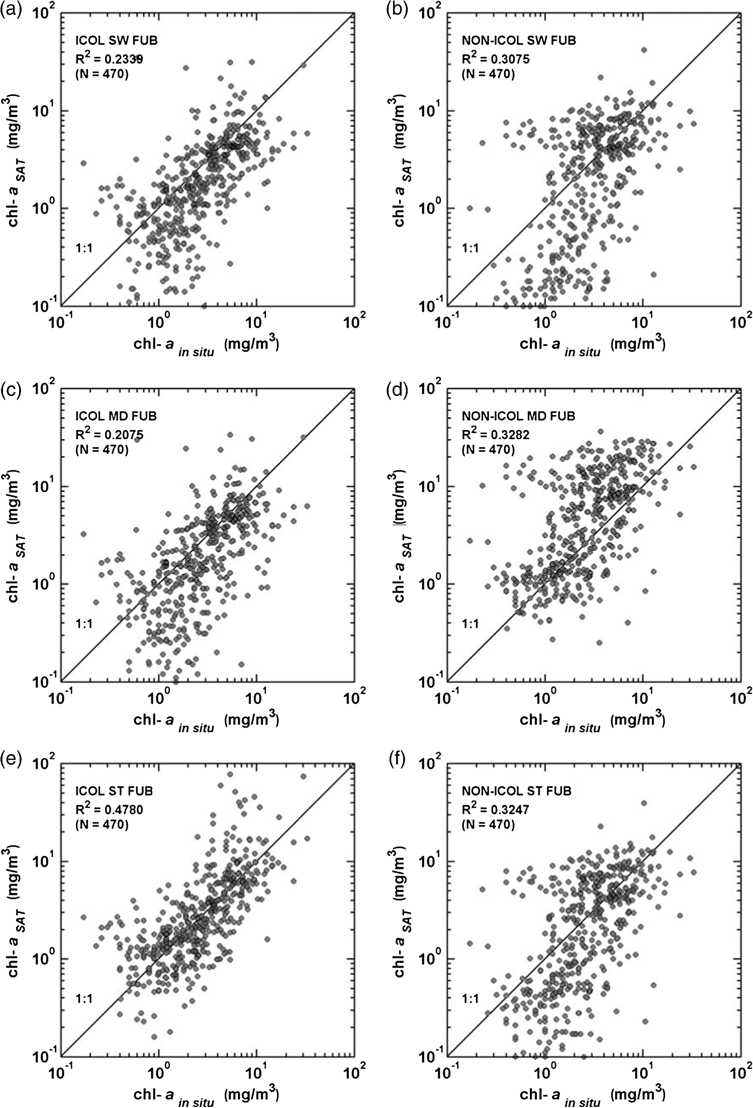

3.3.

Comparison of the chl-a Products Calculated for Coastal Zones and Open Seas

Second, we checked the algorithm accuracy at various locations: coastal and open sea waters (as defined in Sec 2.1) without and with ICOL corrections. All sampling points were grouped according to their location. Improvement in accuracy after applying ICOL was expected in coastal waters where the adjacency effect can occur. However, our results show that ICOL processing only improved MD_FUB and SW_FUB products (by about 150% and 200%, respectively), but ICOL correction did not change the results of standard chl- $a$ concentration products of the FUB processor—ST_FUB (Table 5). However, ICOL_ST_FUB still produced the lowest error in coastal areas. The results obtained with the C2R processor were even much worse after using the ICOL processor (up to 120%) than without this correction. To summarize, the most accurate results for the coastal zone were noted for the standard FUB processor chl- $a$ concentration product either with or without ICOL correction. In the open sea, area ICOL correction improved the algorithms of the C2R processor (ST, MD, and SW) slightly, but it had almost no impact on the algorithms of the FUB processor. Still, the highest accuracy was observed for two band ratio algorithms with the FUB processor: MD_FUB and SW_FUB (Table 5).

Table 5

Comparison of systematic (〈ε〉) and statistical errors (σε) of chlorophyll a concentrations derived from satellite data, using both processors—C2R and FUB, and all algorithms tested (ST, MD, SW) with or without ICOL correction with respect to location (coastal zone or open sea).

Arithmetic statistics for coastal stations $No . of data = 173$					Arithmetic statistics for open sea stations $No . of data = 297$
	NON-ICOL		ICOL		NON-ICOL		ICOL
	$〈 ε 〉$ [%]	$σ_{ε}$ [%]	$〈 ε 〉$ [%]	$σ_{ε}$ [%]	$〈 ε 〉$ [%]	$σ_{ε}$ [%]	$〈 ε 〉$ [%]	$σ_{ε}$ [%]
STC2R	171	459	214	586	186	442	157	373
MDC2R	4	215	25	291	21	202	6	169
SW C2R	27	229	51	306	40	217	25	183
MD FUB	40	422	62	273	$- 16$	81	$- 15$	81
SW FUB	46	474	65	285	$- 13$	77	$- 12$	78
ST FUB	54	171	40	172	48	205	48	206

4. Discussion

Vaiciute¹ observed a connection between the accuracy of the algorithms dedicated for Case-2 waters of MERIS data and Secchi depth. At Secchi depths greater than 3 m, the accuracy was much worse than for shallower values of this parameter. Assuming that such low values of Secchi depth are observed mostly in coastal waters, the results of Vaiciute¹ are also confirmed by our results. In coastal waters, the CDOM concentration is usually higher and can significantly influence the values of water-leaving reflectance, and, thus, the derived concentrations of water components. Generally, the FUB processor produced better results than did the C2R processor, which has also been confirmed in other papers.¹^,¹³^,²¹ In all the cases studied, the MD and SW algorithms produced very similar results. This means that both MD and SW can be applied with similar error results for MERIS and OLCI data in the future. The accuracy of chl- $a$ concentration retrieval is much better in open sea waters, especially for the MD_FUB and SW_FUB algorithms. In these cases, the difference in the relative statistical error between coastal and open sea waters was about 200% after using the ICOL processor and even $> 300 %$ without it (Table 5). As in the case when all data were taken into consideration, there was no improvement after applying ICOL for the C2R processor either in coastal or open sea waters. Even for the algorithms with the best results, the error was still significant, which suggests the necessity of further work on this subject. The spectral resolution of satellite images is currently becoming higher and higher. The possibility of using hyperspectral images allows one to use more spectral bands as input to the algorithms. The accuracy of an algorithm is influenced by many factors resulting from the differences between sampling and satellite image recording. The problems linked to the correct validation of satellite products, for example, chl- $a$ concentration products, are caused by many factors. In order to compare in situ and satellite data, the samples should be collected during satellite overpasses. Accounting for the frequency of the cloudiness over the Baltic Sea, such measurements are not easy to plan or perform. According to Vaiciute,¹ the time of sampling influences the validation results. In this work, the satellite images were recorded on the same day as the samples were taken without accounting for the time of data sampling. Another source of error is that, during algal blooms, especially summer cyanobacterial blooms, the algae in the surface layer are not distributed homogeneously, but form so-called patches that are clearly VIS in satellite images, but difficult to detect in in situ datasets.³² Moreover, when an in situ sample is taken, the algae from the surface are often dispersed by the ship. In our work, we analyzed the images with a spatial resolution of 1.2 km. The analyzed radiance was the mean value of the signal from ${1.44 km}^{2}$ and was compared with the data taken from one point located within the area of the pixel. The influence of this factor is impossible to assess without knowing the characteristic scales of the temporal and spatial variability of chl- $a$ concentrations in the analyzed water basin, both in the coastal zone and further offshore. Finally, as mentioned in Sec. 2.2, the values of chl- $a$ concentrations measured by spectrophotometrical and HPLC methods can vary.¹²^,³¹ This fact can also influence validation results, especially since most of the algorithms for the satellite data have been calibrated by using the HPLC results.¹²

5. Summary

Chl- $a$ MERIS products calculated with two processors were taken into consideration in this study. The FUB processor showed better results than did C2R. The algorithms proposed in the DESAMBEM project, originally designed for SeaWiFS (SW) and MODIS (MD) sensors but adapted to local conditions, were tested for the MERIS data as well. In all cases, the band ratio algorithms (MD and SW) showed similar results. Therefore, it is proposed that both MD and SW can be used with similar error for MERIS and, in the future, OLCI data. These data can be used as a tool for mapping chl- $a$ concentrations in the surface waters of the Baltic Sea. The results show that the adjacency effect can be reduced by processing images with the ICOL for the output of the FUB processor. Moreover, the assessment of the chl- $a$ concentration based on the MERIS images is better for the data located $> 10 km$ from the coast. The significant error obtained suggests the necessity for further work on this subject. In our work, we focused on the variability of chl- $a$ concentrations depending on the location. The concentration of optical properties can change based on the location because of the adjacency effect as well as different ratios between CDOM and chl- $a$ . The variation of the ratios mentioned can influence seasonal variability, which should be considered in future studies. According to this work, the most accurate algorithm for the coastal zone is the standard chl- $a$ concentration product of the FUB processor either with or without ICOL correction. In the open sea area, the highest accuracy was observed for two band ratio algorithms: MD_FUB and SW_FUB (Table 5).

Acknowledgments

This work was carried out within the framework of the SatBałtyk project funded by the European Union through the European Regional Development Fund (contract No. POIG.01.01.02-22-011/09 entitled “Satellite Monitoring of the Baltic Sea Environment”), and also as a part of the system project “InnoDoktorant—Scholarships for PhD students, Vth Edition.” The project is cofinanced by the European Union within the framework of the European Social Fund. The paper was presented in part at the International Geoscience and Remote Sensing Symposium, Melbourne, Australia, 21–26 July 2013.

References

1.

D. VaičiūtėM. BrescianiM. Bučas, “Validation of MERIS bio-optical products with in situ data in the turbid Lithuanian Baltic Sea coastal waters,” J. Appl. Remote Sens., 6 (1), 1 –20 (2012). http://dx.doi.org/10.1117/1.JRS.6.063568 1931-3195 Google Scholar

2.

R. Wasmund, “Occurrence of cyanobacterial blooms in the Baltic Sea in relation to environmental conditions,” Int. Revue Ges. Hydrobiol. Hydrogr., 82 (2), 169 –184 (1997). http://dx.doi.org/10.1002/(ISSN)1522-2632 IRGHAM 0535-4137 Google Scholar

3.

Z. R. Gasiūnaitėet al., “Seasonality of coastal phytoplankton in the Baltic Sea: influence of salinity and eutrophication,” Estuarine Coastal Shelf Sci., 65 (1–2), 239 –252 (2005). http://dx.doi.org/10.1016/j.ecss.2005.05.018 ECSSD3 0272-7714 Google Scholar

4.

J. T. O. Kirk, Light and Photosynthesis in Aquatic Ecosystems, 3rd ed.Cambridge University Press, Cambridge, UK (2011). Google Scholar

5.

J. E. O'Reillyet al., “Ocean color chlorophyll algorithms for SeaWiFS,” J. Geophys. Res., 103 (C11), 24937 –24954 (1998). http://dx.doi.org/10.1029/98JC02160 JGREA2 0148-0227 Google Scholar

6.

W. Schrimpfet al., Thematic Report on Validation of Algorithms for Chlorophyll a Retrieval From Satellite Data of the Baltic Sea Area, 44 (2004). Google Scholar

7.

S. C. LiewA. S. ChiaL. K. Kwoh, “Evaluating the validity of SeaWiFS chlorophyll algorithm for coastal waters,” in Proc. 22nd Asian Conf. on Remote Sensing, 5–9 November 2001, (2001). Google Scholar

8.

J. E. O'Reillyet al., “SeaWiFS postlaunch calibration and validation analyses, Part 3,” SeaWiFS Postlaunch Technical Report Series NASA Technical Memorandum 2000–206892, 11 49 NASA Goddard Space Flight Center, Greenbelt, Maryland (2000). Google Scholar

9.

P. Chauhanet al., “Comparison of ocean color chlorophyll algorithms for IRS-P4 OCM sensor using in-situ data,” J. Indian Soc. Remote Sens., 30 (1–2), 87 –94 (2002). http://dx.doi.org/10.1007/BF02989980 0255-660X Google Scholar

10.

M. KarhuU. HorstmannO. Rud, “Satellite detection of increased cyanobacterial blooms in the Baltic Sea: natural fluctuations or ecosystem change?,” Ambio, 23 (8), 469 –472 (1994). AMBOCX 0044-7447 Google Scholar

11.

M. KahruO. P. SavchukR. Elmgren, “Satellite measurements of cyanobacterial bloom frequency in the Baltic Sea: interannual and spatial variability,” Mar. Ecol. Prog. Ser., 343 15 –23 (2007). http://dx.doi.org/10.3354/meps06943 MESEDT 0171-8630 Google Scholar

12.

M. DareckiD. Stramski, “An evaluation of MODIS and SeaWiFS bio-optical algorithms in the Baltic Sea,” Remote Sens. Environ., 89 326 –350 (2004). http://dx.doi.org/10.1016/j.rse.2003.10.012 RSEEA7 0034-4257 Google Scholar

13.

S. KratzerC. Vinterhav, “Improvement of MERIS level 2 products in Baltic Sea coastal areas by applying the Improved Contrast between Ocean and Land processor (ICOL)—data analysis and validation,” Oceanologia, 52 (2), 211 –236 (2010). http://dx.doi.org/10.5697/oc.52-2.211 OCEGA4 0078-3234 Google Scholar

14.

J. A. Pedrero, Evaluation of MERIS Case-II Water Processors in the Baltic Sea, 120 Helsinki University of Technology, Finland, Espoo(2009). Google Scholar

15.

T. SchroederM. SchaaleJ. Fischer, “Retrieval of atmospheric and oceanic properties from MERIS measurements: a new Case-2 water processor for BEAM,” Int. J. Remote Sens., 28 (24), 5627 –5632 (2007). http://dx.doi.org/10.1080/01431160701601774 IJSEDK 0143-1161 Google Scholar

16.

R. DoerfferH. Schiller, “MERIS Regional Coastal and Lake Case 2 Water Project Atmospheric Correction ATBD,” (2008). http://www.brockmann-consult.de/beam-wiki/download/attachments/1900548/meris_c2r_atbd_atmo_20080609_2.pdf?version=1 Google Scholar

17.

R. DoerfferH. Schiller, “Algorithm Theoretical Basis Document (ATBD) MERIS Lake Water Algorithm for BEAM,” (2008). http://www.brockmann-consult.de/beam-wiki/download/attachments/1900548/ATBD_lake_water_RD20080610.pdf?version=1 Google Scholar

18.

B. Woźniaket al., “Algorithms for the remote sensing of the Baltic ecosystem (DESAMBEM). Part 1: mathematical apparatus,” Oceanologia, 50 (4), 451 –508 (2008). OCEGA4 0078-3234 Google Scholar

19.

M. Dareckiet al., “Algorithms for the remote sensing of the Baltic ecosystem (DESAMBEM). Part 2: empirical validation,” Oceanologia, 50 (4), 509 –538 (2008). OCEGA4 0078-3234 Google Scholar

20.

S. KratzerC. BrockmannG. Moore, “Using MERIS full resolution data to monitor coastal waters—a case study from Himmerfjärden, a fjord-like bay in the northwestern Baltic Sea,” Remote Sens. Environ., 112 (5), 2284 –2300 (2008). http://dx.doi.org/10.1016/j.rse.2007.10.006 RSEEA7 0034-4257 Google Scholar

21.

K. SørensenE. AasJ. Høkedal, “Validation of MERIS water products and bio-optical relations in the Skagerrak,” Int. J. Remote Sens., 28 (3–4), 555 –568 (2007). http://dx.doi.org/10.1080/01431160600815566 IJSEDK 0143-1161 Google Scholar

22.

T. OhdeH. SiegelM. Gerth, “Validation of MERIS Level-2 products in the Baltic Sea, the Namibian coast and the Atlantic Ocean,” Int. J. Remote Sens., 28 (3–4), 609 –624 (2007). http://dx.doi.org/10.1080/01431160600972961 IJSEDK 0143-1161 Google Scholar

23.

R. Santer, Improve Contrast Between Ocean and Land ICOL ATBD Report, 52 (2010) http://cloud.github.com/downloads/bcdev/beam-meris-icol/ICOL_ATBD.pdf Google Scholar

24.

Third Periodic Assessment in the Environment of the Baltic Sea, 1989-1993; Executive Summary, (1996). Google Scholar

25.

H. Mazur-Marzecet al., “Toxic Nodularia spumigena blooms in the coastal waters of the Gulf of Gdańsk: a ten-year survey,” Oceanologia, 48 (2), 255 –273 (2006). OCEGA4 0078-3234 Google Scholar

26.

S. KratzerK. EbertK. Sørensen, “Monitoring the bio-optical state of the baltic sea ecosystem with remote sensing and autonomous in situ techniques,” The Baltic Sea Basin, 407 –435 Springer, Central and Eastern European Development Studies (CEEDES), Berlin (2011). Google Scholar

27.

P. Kowalczuk, “Seasonal variability of yellow substance absorption in the surface layer of the Baltic Sea,” J. Geophys. Res., 104 30047 –30058 (1999). http://dx.doi.org/10.1029/1999JC900198 JGREA2 0148-0227 Google Scholar

28.

S. B. Wozniaket al., “Inherent optical properties of suspended particulate matter in the southern Baltic Sea,” Oceanologia, 53 (3), 691 –729 (2011). http://dx.doi.org/10.5697/oc.53-3.691 OCEGA4 0078-3234 Google Scholar

29.

“ICES data portal,” ocean.ices.dk Google Scholar

30.

International Ocean-Colour Coordinating Group, “Supporting In-Situ Data,” (2011) http://www.ioccg.org/data/insitu.html February ). 2011). Google Scholar

31.

M. DareckiS. KaczmarekJ. Olszewski, “SeaWIFS ocean colour chlorophyll algorithms for the southern Baltic Sea,” Int. J. Remote Sens., 26 (2), 247 –620 (2005). http://dx.doi.org/10.1080/01431160410001720298 IJSEDK 0143-1161 Google Scholar

32.

S. Sagan, “The inherit water optical properties of Baltic waters,” (2008). Google Scholar

33.

“The MERIS Catalogue and Inventory,” http://merci-srv.eo.esa.int/merci/welcome.do Google Scholar

34.

L. BourgL. D'AlbaP. Colagrande, “MERIS smile effect characterization and correction,” (2008) http://earth.eo.esa.int/pcs/envisat/meris/documentation/MERIS_Smile_Effect.pdf June ). 2008). Google Scholar

35.

M. BouvetF. Ramino, “Equalization of MERIS L1b products from the 2nd reprocessing,” (2010). Google Scholar

36.

Th. Schroederet al., “Atmospheric correction algorithm for MERIS above case-2 Waters,” Int. J. Remote Sens., 28 (7), 1469 –1486 (2007). http://dx.doi.org/10.1080/01431160600962574 IJSEDK 0143-1161 Google Scholar

37.

M. WoźniakB. WojtasiewiczK. Bradtke, “Assessment of bio-optical algorithms for satellite radiometers in coastal waters of the Baltic Sea using in situ measurements,” in Abstracts of International Ocean Colour Science Meeting, 253 –254 (2013). Google Scholar

Biography

Monika Woźniak received a BSc degree in mathematics from Szczecin University (Poland) in 2008 and MSc degree in physics from Szczecin University (Poland) in 2007. Currently, she is a PhD student in physical oceanography at the University of Gdansk (Poland). Her PhD project and research interest focus on ocean-color remote sensing of optically complex water in the Baltic Sea.

Katarzyna M. Bradtke obtained her PhD degree at the University of Gdansk (Poland) in 2004. She has been employed at the Institute of Oceanography for 18 years as an associate professor. Her scientific interests focus on satellite data processing using GIS and object-oriented methods. She has published papers which relate to the application of remote sensing in oceanography in Oceanology.

Adam Krężel has had 40 years as an academic teacher at the University of Gdansk, Poland, where he has held, among others, the post of dean of the Faculty of Oceanography and Geography. His research themes are physical oceanography, satellite remote sensing, and marine optics, and he has considerable experience on the international stage, having carried out the measurements of optical parameters in the Baltic and Black Seas and the Atlantic Ocean.

CC BY: © The Authors. Published by SPIE under a Creative Commons Attribution 4.0 Unported License. Distribution or reproduction of this work in whole or in part requires full attribution of the original publication, including its DOI.

Citation Download Citation

Monika Woźniak, Katarzyna M. Bradtke, and Adam Krężel "Comparison of satellite chlorophyll a algorithms for the Baltic Sea," Journal of Applied Remote Sensing 8(1), 083605 (30 June 2014). https://doi.org/10.1117/1.JRS.8.083605

Published: 30 June 2014

Access the abstract

JOURNAL ARTICLE
15 PAGES

DOWNLOAD PAPER SAVE TO MY LIBRARY

GET CITATION

CITATIONS

Cited by 23 scholarly publications.

Explore citations on Lens.org

KEYWORDS

Satellites

Algorithm development

Magnesium

Image processing

Error analysis

Water

Reflectivity

1.

Introduction

2.

Materials and Methods