Hemispheric-scale comparison of monthly passive microwave snow water equivalent products

Jiuliang Liu; Zhen Li; Lei Huang; Bangsen Tian

doi:10.1117/1.JRS.8.084688

22 July 2014 Hemispheric-scale comparison of monthly passive microwave snow water equivalent products

Jiuliang Liu, Zhen Li, Lei Huang, Bangsen Tian

Author Affiliations +

Journal of Applied Remote Sensing, Vol. 8, Issue 1, 084688 (July 2014). https://doi.org/10.1117/1.JRS.8.084688

Abstract

The snow water equivalent (SWE) products from passive microwave remote sensing are useful in global climate change studies due to the long-time and all-weather imaging capabilities of passive microwave radiometry at the hemisphere scale. Northern Hemisphere SWE products, including products from the National Snow and Ice Data Center (NSIDC) and GlobSnow from the European Space Agency (ESA), have been providing long-time series information since 1979. However, the different algorithms used to produce the NSIDC and GlobSnow products lead to discrepancies in the data. To determine which product might be superior, this paper assesses their hemisphere-scale quality for the time period 1979−2010. By comparing the data with historical snow depth measurements obtained from 7388 meteorological stations in the Northern Hemisphere, the accuracies of the different SWE products are analyzed for the period and for different snow types. The results show that for SWEs above 30 mm but below 200 mm, GlobSnow estimates maintain a better linear relation with the ground measurements. NSIDC products are more influenced by microwave “saturation,” producing obvious underestimations for SWEs over 120 mm. However, for shallow snow (SWE less than 30 mm), the slight overestimate produced by GlobSnow is more obvious than that of the other NSIDC products.

1. Introduction

The snowpack is important both as a boundary condition on the atmosphere and as storage for fresh water. The snowpack directly affects climate dynamics and the ecology of cold regions in particular. Therefore, our ability to acquire frequent, high quality, reliable data on the global snow coverage and the volume of water stored in the seasonal and permanent snowpack influences our ability to monitor changes in the climate and to understand the climate system. Although considerable progress has been made recently in determining trends and variability (including quantifying the statistical uncertainty) in snow extent datasets, an adequate understanding of the snow water equivalent (SWE) remains elusive.¹^–³

The SWE is equal to the mass of water per unit area that would be produced if the snowpack was to melt in place. SWE is a product of the snow depth multiplied by the snow density and is generally the preferred measure of snow depth. Recently, gridded SWE products have been produced using interpolations of ground-based observations,⁴^–⁶ atmosphere reanalysis datasets,⁷ general circulation models (GCMs),⁸^,⁹ and various inversions of values obtained from satellite data.¹⁰^,¹¹ However, none of these methods are able to balance the need for better precision and larger spatiotemporal coverage. For climate applications, the SWE values retrieved from satellite passive microwave data are suitable for global large-scale monitoring and temporal analysis because of the wide swath of these data, the all-weather imaging capabilities of the passive microwave radiometry (PMR), and PMR’s multifrequency response to the presence of snow on land. In addition, continuous time series of these data are available dating back to 1978, including sources such as the scanning multichannel microwave radiometer (SMMR) from 1978 to 1987, the special sensor microwave imager (SSM/I) from 1987 to 2007, and the advanced microwave scanning radiometer-EOS (AMSR-E) from 2002 to 2011.

Inversion algorithms based on PMR have been developed and improved to produce several global-scale SWE products. Early SWE retrieval approaches depended on the linear relationship between snow depth and the brightness temperature difference between two channels operating at different frequencies (usually near the Ka band at 19 GHz and the K band at 37 GHZ obtained from PMR).¹¹ This approach was used because the radiation intensity received by PMR is emitted from soil and will be scattered and attenuated by the snowpack in snow-covered areas. The higher the frequency is, the greater the apparent attenuation.¹² Snow grain size is the major source of error in SWE estimates because microwave radiation is sensitive to this factor. Increasing grain size has a positive influence on scattering and, therefore, the SWE is overestimated if the algorithm considers it as a constant (0.3 mm). In reality, snow grain sizes vary considerably with time and location. The snow grain size often grows during the compaction process as the snowpack becomes deeper or forms depth hoar.¹³ Vegetation is another major source of error in the SWE estimates.¹⁴ The vegetation layer masks the signal of the underlying snowpack via scattering and absorption. The SWE tends to be significantly underestimated if the forest cover density exceeds 30%–40% and the degree of underestimation can reach 50% in the densely forested areas of Canada.¹⁵ The forest fraction is often used to systematically adjust this underestimation in global retrievals of SWE. However, parameters, such as stem volume or canopy closure, are theoretically more capable than the forest fraction of describing the impact on the emitted radiation.¹⁶ Most seasonal snow covers are found in boreal forest areas; thus, this problem is inevitably encountered by global SWE retrieval algorithms.¹⁷ Wet snow is usually identified using a brightness threshold, and the amount of liquid water cannot accurately be estimated via passive microwave signals because the influence of water in the snow leads to a completely saturated brightness temperature response once the liquid water fraction reaches 10%.¹⁸ The influences of the atmosphere and topography are of less concern.¹⁹

Based on these influences, current global-scale algorithms are applied in dry snow areas, and impossible to retrieve pixels, such as those corresponding to mountains and areas of wet snow, are excluded. Published global SWE products derived from SMMR & SMM/I and AMSR-E data are released by the National Snow and Ice Data Center (NSIDC), and their algorithms include modified versions of Chang’s brightness temperature difference algorithm. The two NSIDC products are referred to as NSIDC (SMMR & SSM/I)²⁰ and NSIDC (AMSR-E)²¹ in this paper. Comparisons of Chang’s retrieval algorithm and the station SWE datasets from the former Soviet Union indicate that the algorithm has a general tendency to underestimate the snow water equivalence, especially in densely forested areas. However, the systematic errors in the results produced using this method when compared with the validation data are fairly constant and, thus, this method is capable of detecting temporal changes in the SWE.¹⁶ The NSIDC (SMMR & SSM/I) and NSIDC (AMSR-E) introduced the global forest fraction dataset into their algorithms with the intent of minimizing the vegetation influence.

In contrast, some advanced studies have attempted to introduce microwave radiation models into the retrieval process with the aim of better predicting the microwave radiation from the snowpack based on physical mechanisms.²²^–²⁶ These methods often have higher precision but are too complex for direct retrieval of snow variables under varying snow conditions at the hemisphere scale. Among these methods, the HUT model (developed at Helsinki University of Technology) is an adequate simple model that has proven feasible in global SWE retrieval. This method effectively simulates emitted radiation by considering the contributions from a single-layered homogenous snowpack, the vegetation cover, and the atmosphere via empirical methods and combining them into the total model. A Bayesian inversion method for the HUT emission model²⁷^–²⁹ has proven to be more accurate, with a lower root-mean-square error (RMSE) and bias than those of other algorithms³⁰ (including the NSIDC operational algorithm²⁰ and the AMSR-E standard SWE product²¹) when applied over Eurasia, Canada, and northern Finland. This so-called FMI (Finnish Meteorological Institute) algorithm has been developed further, resulting in an advanced process known by its SWE product, GlobSnow³¹. Some studies have confirmed that GlobSnow has the advantage of being able to estimate peak snow accumulation, as well as derive seasonal patterns in SWE values. ³² However, occasional abrupt changes in the values seen in the daily (v1.0 and v1.2) and weekly (v1.2) products have been reported, even though this method uses two pixel observations.³³

A problem associated with both the brightness temperature difference algorithms and the assimilation algorithm is that it is difficult to determine their accuracy. Thus, there is a lack of reliable quantifiable indices for SWE product selection in practical applications. Until now, no comparisons have been performed at the global-scale and over long time periods. In this paper, we describe the comparison between a large set of snow depth measurements from meteorological stations and three PMR products, such as GlobSnow and the two NSIDC SWE products. The comparison was made for the Northern Hemisphere for the period 1978–2010 and provides an assessment of the scope of application of these products for SWE retrieval. Because the PMRs’ brightness temperature is influenced by the properties of the snow (i.e., the amount of snow, snow grain size, snow density, and the presence of liquid water), it is necessary to make comparisons for similar snow classes, which are defined according to the properties of the snow.

2. Data

2.1.

Satellite-Retrieved Monthly Snow Water Equivalent Products

2.1.1.

NSIDC (SMMR & SSM/I) snow water equivalent product

This product consists of global monthly SWE derived from SMMR data spanning the period from 1978 to 1987 and SSM/I data from 1987 to 2007. These data are gridded to the northern 25-km equal-area scalable Earth grids (EASE-grids)²⁰ and released by the NSIDC. The SWE is derived for pixels in which visible snow was observed in the EASE-grid weekly snow cover and sea ice extent Version 2 data at least once during the month under study. Pixels from the 25-km EASE-grid version of the BU-MODIS land cover data that have more than 50% ice cover are set as permanent ice without SWE inversion values.

The classical Chang algorithm makes use of a brightness temperature difference to estimate the SWE and is implemented in this product as follows:

Eq. (1)

SMMR : SWE [mm] = 4.77 * ({Tb}_{18 H} - {Tb}_{37 H}),

Eq. (2)

SSM / I : SWE [mm] = 4.8 * ({Tb}_{19 H} - {Tb}_{37 H} - 5),

where

{Tb}_{18 H}

(

{Tb}_{19 H}

) and

{Tb}_{37 H}

are the brightness temperatures for the horizontal polarizations at 18 (19) and 37 GHz, respectively. For SSM/I data, the 19-GHz frequency takes the place of 18 GHz on the SMMR, and an adjustment of

- 5

is made to the spectral difference. Two important approximations are made. First, the snow grain size is assumed to be a constant 0.3 mm, and second, the snow density is set to a constant

0.3 g / {cm}^{3}

. For pixels covered by forest, an adjustment is made using the forest fraction, and the final SWE is written as

Eq. (3)

{SWE}_{adjust} = SWE / (1 - F) .

In this work, the value of $F$ is defined according to the forest fractions in the 25-km EASE-grid version of BU-MODIS land cover. Specifically, $F$ is equal to the forest fraction except when the forest fraction is greater than 50%, in which case the value of $F$ is set to 0.5.

2.1.2.

NSIDC (AMSR-E) snow water equivalent product

The AMSR-E L3 Global SWE is a global monthly inverted SWE product based on the brightness temperatures from AMSR-E covering the period from June 2002 to October 2011. This product is also projected onto a 25-km EASE-grid at the hemisphere scale and is available on the NISDC website.²¹ The land cover, ocean, and ice-sheet masks used are based on the EASE-grid version of MODIS land cover data, MOD12Q1 IGBP. Pixels that are assumed to represent wet snow, mountains, rain, or other impossible pixels are excluded before SWE retrieval.

The algorithm used to produce this product is derived from Chang’s brightness temperature difference method. However, with the availability of the special X-band channels on AMSR-E at 10.7 GHz, the algorithm’s ability to detect deep snow (using the difference between 10.7 and 18.7 GHz) is improved and its dynamic range is enhanced to aid in forest attenuation.³⁴ The snow depth is estimated using the equation

Eq. (4)

SD = ff * {SD}_{f} + (1 - ff) * {SD}_{o},

where SD is the total sample snow depth,

{SD}_{f}

and

{SD}_{o}

are the snow depths in the forested and nonforested components of the instantaneous field of view, respectively, and

ff

is the forest fraction ranging from 0% to 100% obtained from the MOD12Q1 IGBP data. The forested snow depth (

{SD}_{f}

) and nonforested snow depth (

{SD}_{o}

) can be calculated as follows:

Eq. (5)

{SD}_{0} [mm] = 1 / \log_{10} ({pol}_{36}) * ({Tb}_{18 V} - {Tb}_{36 V}) / (1 - f d * 0.6),

Eq. (6)

{SD}_{f} [mm] = [1 / \log_{10} ({pol}_{36}) * ({Tb}_{18 V} - {Tb}_{36 V})] + [1 / \log_{10} ({pol}_{18}) * ({Tb}_{10 V} - {Tb}_{18 V})],

where

f_{d}

is the high spatial resolution (500 m) forest density obtained from the University of Maryland MODIS vegetation continuous fields (VCF) (GLCF_MODIS_VCF) ( http://glcf.umiacs.umd.edu/data/vcf/). Both of the estimated forest variables (fraction and density) are circularly smoothed at a diameter of 15 km and regridded globally at 1 km. The

{Pol}_{18}

and

{Pol}_{36}

are the brightness temperature differences between the vertical and horizontal channels at 18.7 and 36.5 GHz, respectively. Note that if either

{Pol}_{18}

or

{Pol}_{36}

is less than 1.1, then

{Pol}_{36}

is set to 1.1 to ensure that the value of the logarithm is greater than zero. Finally, the estimated SWE values for the 25-km pixels can be obtained by multiplying the SD by the snow density. The snow density employed in this product is obtained from a global snow density map, in which the average snow density value for each of the six seasonal classes is calculated according to in situ measurements collected in Canada³⁵ and the former Soviet Union.³⁶

2.1.3.

GlobSnow snow water equivalent products

The GlobSnow SWE product (Version 1.3) for the Northern Hemisphere provides information on the SWE obtained using the SMMR, SSM/I, and AMSR-E sensors combined with ground-based weather station data from 1979 to 2011. This product is one of the products that comprise the European Space Agency (ESA) data user element (DUE) GlobSnow project and is also stored in the EASE-grid format ( http://www.GlobSnow.info/). All land surface areas are covered, except for mountainous regions and Greenland, based on a mask derived from a $2^{'} \times 2^{'}$ grid of ETOP2 data, which contain global elevation and bathymetry from the National Geophysical Data Center (NGDC).³⁰

The GlobSnow SWE is retrieved using an assimilation scheme based on a semiempirical HUT snow emission model, which uses the brightness temperature combined with ground-based measurements from meteorological stations (obtained from the ECMWF). The HUT model considers emissions at frequencies of 11 to 94 GHz to be affected by the atmosphere, forest cover, and a single-layer homogenous snowpack that covers frozen ground, all of which are modeled separately using an empirical approach and which constitute the overall model. Snow variables, including SD/SWE, grain size, and snow density, describe the influence on the radiation emitted by the snow. The SWE estimate is obtained by minimizing the differences between the observed and modeled values of the brightness temperature differences for a set of snow variables, as well as the difference between the estimated and prior values of snow depth.

In practice, the retrieval process consists of three steps. First, the effective snow grain size at the reference stations, in which the snow depth is observed, is estimated. Second, a kriging-interpolated background map of the effective snow grain size (prior) is constructed, as well as a coarse estimate of snow depth or SWE (prior) derived from a set of ground-based observations. Third, the SWE is produced by comparing the satellite Tb observations and the HUT model Tb simulations by weighting the two data sources according to the variance in their respective estimates using the interpolated effective grain size produced in the previous step. The final SWE (posteriori) is optimized as follows using a Bayesian approach:

Eq. (7)

\min_{D_{t}} {{(\frac{({Tb}_{19 V, \mod} (D_{t}) - {Tb}_{37 V, \mod} (D_{t})) - ({Tb}_{19 V, obv} (D_{t}) - {Tb}_{37 V, obs} (D_{t}))}{σ_{t}})}^{2} + (\frac{(D_{t} - {\overset{͡}{D}}_{ref, t})}{λ_{D, ref, t}})},

where

{\overset{͡}{D}}_{ref, t}

and

λ_{D, ref, t}

are the mean snow depth and standard deviation of the snow estimated from the integrated map, respectively.

{Tb}_{19 V}

and

{Tb}_{37 V}

denote the vertically polarized brightness temperatures at 19 and 37 GHz, respectively, with the respective subindices mod and obs referring to the HUT-modeled and observed values. This process is fully described in the paper by Pulliainen.²⁹ In addition, areas that are identified as snow covered by Takala’s time series melt-detection algorithm, but for which an SWE estimate is not produced, are set to a marginal SWE value (0.001 mm) in the final SWE product.³⁷

The daily effective grain-size map used in this product is dynamically changed according to the real-time station measurements. The snow density is treated as a constant with a value of $0.24 g / {cm}^{3}$ , which is a reasonable “global” value given by the analysis of Sturm.³⁸ The forest inventory variables used in the HUT model are forest fraction and stem volume, with the forest fraction values taken from GLC2000 (Global Land Cover classification 2000).³⁹ Although the stem volume has not been considered in the version currently released, relative modifications have been made in test versions (private communication with Kari Luojus).

2.2.

Ground Meteorological Station Measurements

2.2.1.

GHCN-daily measurements data

A hemisphere-scale comparison of SWE products requires large quantities of ground truth data that include as many measurements from across the world as possible to preserve continuity and to avoid accidental errors introduced by the use of single measurements to represent the average values of large pixels. The consecutive records of snow depth measurements that can be found in the Global Historical Climatology Network (GHCN)-daily dataset on the NOAA website meet our spatial and temporal needs. The GHCN-daily dataset is an integrated database of daily climate summaries from land surface stations across the globe that are produced using more than 20 sources of data. Daily variables (i.e., total daily precipitation and maximum and minimum temperatures) from a total of over 79,834 stations in 180 countries and territories are integrated and subjected to a common suite of quality assurance reviews. The snow depth data are provided by 29,814 stations (all marked with a colored cross in Fig. 1) covering different continuous time spans. Since the 1980s, the stations that provide snow depths and the consistency of their records have been enhanced, especially in the case of the stations in North America, northern Europe, and Siberia. These GHCN-daily data can be obtained from NOAA at http://www.ncdc.noaa.gov/oa/climate/ghcn-daily/index.php. However, snow density is not one of the parameters included in this dataset. In practice, snow depth is converted into SWE using the uniform value for snow density used in the different products derived from satellite data.

Fig. 1

Locations of the GHCN-daily meteorological stations. The crosses indicate the 29,814 stations that provide snow depth measurements for 1979–2010, and these are colored according to the seasonal snow classification (i.e., the six snow classes known as tundra, taiga, maritime, ephemeral, prairie, and alpine).⁴⁰ The points denote the selected stations and at each of these, there were at least 15 days of snow cover in the month studied.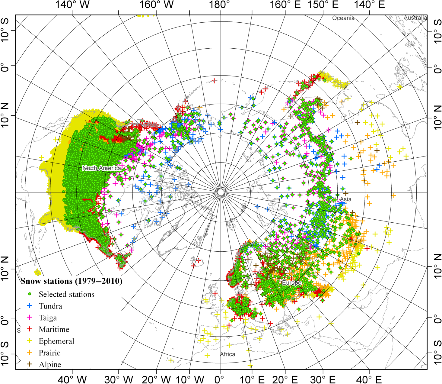

2.2.2.

Ground measurement data selection

Before the ground truth data could be used in the evaluation of the monthly retrieved SWE products, it was necessary to eliminate invalid values from the GHCN-daily datasets and to convert the daily measurements to monthly averages. In the projection conversion operation, all the GHCN-daily meteorological stations were projected onto the EASE-grid projection. Only the pixels that featured simultaneous collection of both the ground measurements and the observations used to produce the GlobSnow and NSIDC products were selected. If two or more stations were located within a single pixel, their average value was taken as the value of that pixel. In addition, the meteorological stations that are used in the GlobSnow assimilation algorithm were eliminated from the GHCN-daily datasets to maintain the fairness of the evaluation. Finally, we selected 7388 meteorological stations in the GHCN-daily database (points in Fig. 1). For each of these stations, there were at least 15 days of snow cover in the month, and the mean depth is thus referred to as the “monthly GHCN measurement.”

The “monthly GHCN measurement” had to be converted into the required “ground-measured SWE” to evaluate the monthly retrieved SWE values from the three products. The most common method is to multiply the measured snow depth by the snow density. Because the snow density values used in the three products are different [ $0.24 g / {cm}^{3}$ in the case of GlobSnow, $0.3 g / {cm}^{3}$ in the case of NSIDC (SMMR & SSM/I), and average density values for each of the six snow classes³⁸ in the case of NSIDC (AMSR-E)], the “ground-measured SWE” datasets were calculated separately for each product.

3. Results

3.1.

Overview of Satellite-Retrieved Monthly Snow Water Equivalents

For the retrieval products, the SWE maps of the Northern Hemisphere from NSIDC (SMMR & SSM/I), NSIDC (AMSR-E), and GlobSnow display completely different spatial distributions, primarily due to their use of different algorithms. Taking the climatological monthly SWE distributions as an example, it is clear that the patterns of SWE values including the locations of highest SWE (or greatest snow depths) contain dissimilarities at the hemisphere scale (Fig. 2).

Fig. 2

The Northern Hemisphere monthly SWE data and the corresponding monthly average air temperature in January 2003. (a)–(c) are SWE data from NSIDC (SMMR &SSM/I), NSIDC (AMSR-E) and GlobSnow in January 2003, respectively, including the detectable snow cover areas of these different retrieval processes. The data in (d) are obtained from the gridded dataset “GHCN_CAMS Gridded 2m Temperature (Land)” (0.5 deg latitude × 0.5 deg longitude) in January 2003.

In terms of coverage, both NSIDC products extend to lower latitude regions, especially over Eurasia, whereas the GlobSnow products cover a smaller area. To avoid topographic influences, GlobSnow excludes additional mountain areas, such as the Tibetan plateau and the Rocky Mountains, in its retrieval process.

Both NSIDC products exhibit greater SWE values over Siberia and lower values over western Eurasia, whereas the GlobSnow SWE algorithm map locates the maximum SWE (or snow depth) in western Siberia. The locations of the greatest SWE estimates in the NSIDC products are exactly the same as those of the coldest locations at the time. This result is believed to be caused by variations in snow grain size, which are influenced by the low air temperatures. In the Chang-based static algorithms, the coefficient between the brightness temperature differences and the SWE actually represents an index of relative grain size growth. At air temperatures well below freezing, e.g., those occurring in Siberia in winter, temperature gradient metamorphism greatly accelerates the snow grain growth.⁴¹^,⁴² The value of this coefficient may, therefore, change and using a constant value for this coefficient, as is done in the NSIDC algorithms, will not reflect these variations. This effect has been confirmed by a dynamic simulation result that attributed the growth in snow grain size to the temperature gradient metamorphism and successfully corrected the locations of the maximum SWE values westward in central Siberia,⁴¹ similar to the situations shown in the GlobSnow SWE map [Fig. 2(c)]. In addition, previous studies have also shown that the Chang-based static algorithms tend to overestimate SWE to a greater extent than the GlobSnow does when the cold air temperature is particularly low( $< - 35 ° C$ ).⁴³ However, the global effective grain size maps that are used in the GlobSnow retrieval process are produced every day upon request. The effective grain size not only acts as a physical equivalent parameter of crystal size but also includes many environmental factors (e.g., liquid water content, soil temperature variations, physical snow grains, etc.) that affect the relation between the SWE and microwave signals. Therefore, GlobSnow has the advantage of being able to reduce these errors caused by snow metamorphism.⁷

3.2.

Perspective on the Mean Difference Between Snow Water Equivalent Products and Ground Measurements

An overall assessment of the algorithm performance was further achieved by comparing SWE retrievals with the reference to “ground-measured SWEs,” which were derived from “GHCN measurements” in this study, for the entire period of the SWE products’ validity in the Northern Hemisphere. Figure 3 contains a histogram that shows the biases of the three products from each November to the following April during the period of validity of the products and also shows the degree of dispersion in the estimates derived from the three different satellite products. Compared with the two NSIDC products, the degree of discrete deviation between the GlobSnow SWE product and the “ground-measured SWE” is smaller. More of the biases in both NSIDC products (especially NSIDC (AMSR-E)) are negative, which means that the NSIDC products are more likely to underestimate SWE.

Fig. 3

Histogram of biases between satellite-derived SWEN (or SWEG) and ground-measured SWET: (a) SWE from NSIDC (SMMR&SSM/I) and GlobSnow in the period 1979–2010 (the number of samples is 139,877) and (b) SWE from NSIDC (AMSR-E) and GlobSnow in the period 2002–2010 (the number of samples is 21,501).

Figure 4 presents the mean differences between the derived SWE products and “ground-measurement SWE” for all selected meteorological stations for the entire period of availability of the SWE products for the snow-covered area of the Northern Hemisphere. In general, cases of extreme overestimation or underestimation by GlobSnow are very few and they are widely separated, without any regional concentration. In the area of extreme cold, i.e., Siberia, both NSIDC products detect higher values of SWE than those acquired by meteorological stations (most measurements are higher by at least 50 mm); whereas in western Eurasia, the NSIDC products detect values that are much lower than those acquired by the meteorological stations (in most cases the difference is again at least $- 50 mm$ ). These observations are completely consistent with the misallocation of deeper snow in the Eurasian areas of extreme cold shown in Fig. 2. The reason for this possible induced error is discussed in Sec. 3.1.

Fig. 4

Northern Hemisphere mean difference distribution. The differences shown are between the following: (a) NSIDC (SMMR&SSM/I) SWEN and ground-measured SWET in the period 1979–2010; (b) GlobSnow SWEG and SWET in the period 1979–2007; (c) NSIDC (AMSR-E) SWEN and SWET in the period 2002–2010; (d) GlobSnow SWEG and SWET in the period 2002–2010.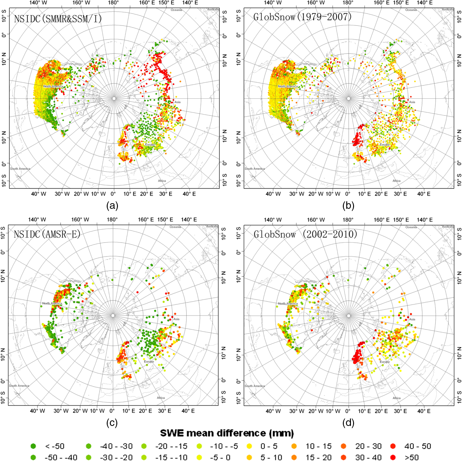

In North America, the SWE estimates are higher than the station measurements in eastern Canada, where the snow is classified as being maritime snow. This is the case for all three satellite-derived SWEs but is more obvious for the NSIDCs products. Foster¹⁵ attributed the overestimates partly to the presence of open water bodies, which contaminate pixels in the maritime snow class and affect passive emission and also the air temperature. This generally warmer region [where the temperature is approximately 0°C even in January, as shown in Fig. 2(d)] tends to have wetter snow, which results in there being less attenuation of satellite-received radiation at a frequency of 37 GHz and thus smaller brightness temperature differences. The SWE is, therefore, underestimated. The SWE values from the meteorological station measurements agree quite well with retrieved estimates over the Canadian prairies, and this result was also reported by Brown⁴⁴ and Mote.⁴⁵ The Scandinavian Peninsula is an exception in that all SWE estimates are larger than the in situ measurements; unfortunately, the underlying reason for this is not clear.

3.3.

Global Analysis of Correlation and Retrieval Errors for Satellite-Derived Snow Water Equivalents

The accuracies of the GlobSnow SWE and the two NSIDC SWE products were also assessed by comparing the results with various measured snow depths to illustrate the correlation and magnitude of the differences between the snow depths and the derived SWE products. Table 1 shows the results obtained for this accuracy testing. To display the trends more clearly, accumulations are displayed in 5-mm steps in Fig. 5. It is obvious that the estimated SWE, as produced by all three products, does not increase monotonically with increasing snow depth.

Table 1

Correlation (Coor), root-mean-square error (RMSE), standard deviation (SD), and bias for the relation between “ground-measured SWE” and satellite-derived SWEs in the Northern Hemisphere.

Global	$0 < SWE < 30 mm$				$30 mm < SWE < 200 mm$
Global	Coor	RMSE/mm	Std/mm	Bias/mm	Coor	RMSE/mm	Std/mm	Bias/mm
SMMR&SSM/I	0.23	28.07	21.07	10.97	0.24	62.23	34.39	$- 27.01$
GlobSnow(1979–2007)	0.21	43.13	28.78	22.58	0.62	35.27	21.41	$- 12.57$
AMSR-E	0.26	29.08	15.24	17.58	0.13	54.90	19.26	$- 29.61$
GlobSnow(2003–2010)	0.16	62.20	30.68	43.18	0.55	38.86	19.34	$- 16.35$

Fig. 5

Comparisons of “ground-measured SWE” and the satellite-derived SWE for the complete time period of each product: (a) SWE from NSIDC (SMMR & SSM/I) and GlobSnow (the number of samples is 139,877); (b) SWE from NSIDC (AMSR-E) and GlobSnow (the number of samples is 21,501).

Compared with the two NSIDC products, a better linear relationship exists between GlobSnow SWE and “ground-measured SWE” for values over 30 mm, and GlobSnow provides a clear improvement in retrieval accuracy (lower RMSE, standard deviation and bias). The correlation coefficients are 0.62 (Table 1) for the period from 1979 to 2007 and 0.55 for the period from 2002 to 2010. The underestimation of the SWE by the NSIDC products becomes clear for values over around 120 mm (Fig. 5) and, in this case, the correlation coefficients are only 0.22 and 0.13 for the same two periods, respectively. However, an inevitable underestimation exists in all of the products due to the high-frequency microwave “saturation” in deep snow. Theoretically speaking, because the microwave upwelling radiation emitted from the ground by scattering no longer decreases with increasing snow depth at higher microwaves frequencies (37 GHz), passive microwave SWE retrieval algorithms do not have the ability to detect deep snow and thus have a documented tendency to systematically underestimate the SWE in such conditions. When SWE values exceed a certain threshold, the snowpack experiences a transition from acting as a scattering medium to being a microwave emission source.³⁷ Previous studies have shown that this observable scattering saturation for thick snow packs was often achieved beyond a certain threshold of approximately 100 mm for the NSIDC products. However, with the abundant site measurements of snow depth assimilated into GlobSnow’s inversion process, the GlobSnow SWE threshold was greater than approximately 150 mm³²^,⁴²^,⁴⁶ and was perhaps even as high as 200 mm.

For values of SWE of less than 30 mm, the GlobSnow product shows a tendency to overestimate, an effect that is more obviously pronounced than that of the NSIDC products. This overestimation was also observed in previous accuracy testing experiments performed for Eurasia,⁴⁷ but the specific reason for this phenomenon remains unclear. Given the differences in the retrieval algorithms, the most likely explanation is that shallow snow tends to be missed in the assimilation approach in the early or late snow seasons and GlobSnow mistakes the existence of localized deeper snow for continuous snow cover over large areas.³² However, this speculation requires further investigation.

3.4.

Accuracy of Snow Water Equivalent Products for Different Snow Classes

Given the influence of the snow properties on the snow retrievals and the various environments across the global snow-covered area, the accuracy of the SWE products for different snow classes should be discussed. Sturm⁴⁰ categorizes the snowpack in the Northern Hemisphere into six classes: tundra, taiga (the Russian word for the subarctic, moist, coniferous forest), maritime, prairie, alpine, and ephemeral. Each of the six snow classes listed above in Fig. 1 is defined by a unique ensemble of comprehensive characteristics, including snow density, depth, crystal morphology, and grain size features within each snow layer, all of which directly affect the SWE retrievals. To link all of the accuracy results with these classes of each meteorological station, Fig. 6 presents the details of the comparisons between the “ground-measured SWE” and the satellite-derived SWE products for each snow class for the period between 1979 and 2007. The same process was carried out for NSIDC (AMSR-E) and GlobSnow for the period between 2002 and 2010, but the results are not displayed here due to their similarity to the results shown in Fig. 5 and the limited length of this paper. However, the relevant statistical parameters are shown in Table 2 together with those for NSIDC (SMMR&SSM/I).

Fig. 6

Comparisons of “ground-measured SWE” and the satellite-derived SWE for each of Sturm’s snow classes between 1979 and 2007, including (a) Tundra snow, (b) Taiga snow, (c) Maritime snow, (d) Prairie snow, (e) Alpine snow, and (f) Ephemeral snow. The SWE estimates are from NSIDC (SMMR & SSM/I) and GlobSnow.

Table 2

Correlation, standard deviation (Std), root mean square error (RMSE) and bias for the relations between “ground-measured SWEs” and satellite-derived SWEs for Sturm’s snow classes.

		$0 < SWE < 30 mm$				$30 mm < SWE < 200 mm$
		Coor	RMSE/mm	Std/mm	Bias/mm	Coor	RMSE/mm	Std/mm	Bias/mm
1979–2007
Tundra	NSIDC(SMMR&SSM/I)	0.09	58.22	42.81	37.02	0.31	57.72	36.31	$- 5.83$
Tundra	GlobSnow	0.02	67.26	50.89	41.18	0.67	32.40	19.90	$- 3.63$
Taiga	NSIDC(SMMR&SSM/I)	0.18	71.97	41.11	47.84	0.13	72.05	49.73	$- 8.71$
Taiga	GlobSnow	0.07	45.47	17.96	20.76	0.76	28.05	16.92	$- 4.58$
Maritime	NSIDC(SMMR&SSM/I)	0.14	17.80	12.62	2.83	0.09	72.90	16.27	$- 60.83$
Maritime	GlobSnow	0.13	57.82	32.95	33.04	0.44	45.41	22.13	$- 19.32$
Prairie	NSIDC(SMMR&SSM/I)	0.32	23.39	16.62	7.54	0.32	45.59	25.04	$- 23.81$
Prairie	GlobSnow	0.25	27.83	16.66	13.74	0.61	30.17	16.34	$- 12.66$
Alpine	NSIDC(SMMR&SSM/I)	0.23	36.25	22.35	20.37	0.22	61.55	26.83	$- 35.47$
Alpine	GlobSnow	0.21	54.18	27.54	33.71	0.65	34.37	17.70	$- 13.13$
Ephemeral	NSIDC(SMMR&SSM/I)	0.28	8.61	4.84	$- 1.29$	0.11	63.09	8.56	$- 47.53$
Ephemeral	GlobSnow	0.41	6.05	3.17	$- 1.40$	0.65	56.06	4.66	$- 47.81$
2002–2010
Tundra	NSIDC(AMSR-E)	0.15	40.94	19.76	28.03	0.29	46.90	33.99	$- 11.35$
Tundra	GlobSnow	0.11	43.28	16.58	26.81	0.62	32.46	17.51	$- 6.54$
Taiga	NSIDC(AMSR-E)	0.26	31.50	18.85	17.55	0.15	46.69	21.17	$- 18.65$
Taiga	GlobSnow	0.12	37.47	10.87	12.18	0.67	31.35	14.23	$- 9.83$
Maritime	NSIDC(AMSR-E)	0.20	23.76	13.39	14.23	0.19	68.34	13.24	$- 54.84$
Maritime	GlobSnow	0.11	75.00	34.31	52.86	0.41	47.09	21.37	$- 22.12$
Prairie	NSIDC(AMSR-E)	0.37	29.57	14.69	18.66	0.22	38.87	25.05	$- 10.33$
Prairie	GlobSnow	0.27	49.50	19.03	30.53	0.42	37.27	14.91	$- 20.01$
Alpine	NSIDC(AMSR-E)	0.20	33.33	18.37	20.95	0.08	55.70	21.59	$- 33.60$
Alpine	GlobSnow	0.19	63.65	25.55	44.58	0.59	39.31	16.39	$- 21.36$
Ephemeral	NSIDC(AMSR-E)	0.11	5.20	19.58	$- 20.86$	—	—	—	—
Ephemeral	GlobSnow	0.61	4.54	1.58	$- 2.03$	—	—	—	—

Figure 6 shows that the GlobSnow SWE maintains better consistency with ground measurements than NSIDC (SMMR & SSM/I) for all snow classes, and NSIDC (SMMR&SSM/I) appears to produce higher SWE values for the taiga class up to the saturation point. With Table 2, these data show that the correlations between GlobSnow and ground measurements for SWEs less than 30 mm are all smaller than those between the NSIDC products and ground measurements. This situation is reversed for deep snow, similar to what was seen in the global comparisons. The smaller standard deviations and RMSEs in GlobSnow indicate that the errors in the estimates are relatively smaller, regardless of the difference between the retrievals and ground measurements or the deviation of single estimated values. The bias of GlobSnow displays a larger number of positive values for shallow snow and a smaller number of negative values if the SWE is greater than 30 mm.

In Fig. 6, the NSIDC (SMMI &SSM/I) presents obvious systematic overestimates in the taiga snow class, which is characterized by dense forest and deep snow cover. This provides good evidence of the error induced by forest scattering, which produces higher brightness temperature differences. However, the overestimates in NSIDC (AMSR-E) are significantly reduced due to the algorithm that is used and the special 10.7 GHz channel on this instrument (Table 2). Both NSIDC products tend to consistently underestimate SWE values in the case of the maritime snow classes. This observation is consistent with the error distributions described in Sec. 3.2 and is primarily due to the melt features in relatively warm maritime climates. The NSIDC products are more reliable as the snow depth increases on the prairies because vegetation is sparse, and the discrepancies between their values and those of GlobSnow are then minimal. Overestimate of GlobSnow in shallow snow ( $SWE < 30 mm$ ) is a common occurrence for the tundra and alpine classes because tundra and alpine areas, whatever the snow depth, are frequently influenced by wind. In these areas, the meteorological stations are sparsely distributed and topographic influences on the redistribution of snow by the wind can be significant, thus leading to shallow snow that is overlooked in the GlobSnow process.³²^,⁴⁸ Note that the NSIDC overestimate for tundra, in which the SWE is less than 30 mm, is greater than any other class and the error in this case is large. In contrast to the reasons given for GlobSnow, the typically larger basal snow crystals of tundra snow might contribute more to these overestimates.¹⁵ Although ground measurements of ephemeral snow class are rare, better correspondence is observed between these measurements and both the NSIDC and the GlobSnow products for this relatively warm and thin snow class.

4. Conclusion

In this paper, the Northern Hemisphere monthly SWE products NSIDC (SMMR & SSM/I), NSIDC (AMSR-E), and GlobSnow SWE were validated through comparisons with worldwide ground-based measurements of snow depth over the time period 1979 to 2010 to demonstrate the accuracies of the typical stand-alone brightness temperature difference algorithms and assimilation approach used in SWE retrieval.

The spatial mean distribution differences between these retrieved products also highlight the NSIDC static algorithm defects. These problems include mislocating the location of the maximum SWE that occurs in the extreme-cold region of Siberia and underestimating the SWE values in western Eurasia and eastern Canada. In contrast, the station-based assimilation approach of GlobSnow has the advantage of being able to reduce these errors.

The comparisons show that for values of SWE below 200 mm, the abilities of the two NSIDC products and the GlobSnow SWE product to measure SWE differ depending on whether the SWE value is greater or less than 30 mm. For SWEs greater than 30 mm, GlobSnow displays a better linear relationship with the ground measurements, whereas the two NSIDC SWE products are more heavily influenced by the inevitable underestimation due to the “saturation” of high-frequency microwaves in deep snow. For areas with thin snow cover, i.e., with values of SWE less than 30 mm, the overestimation by GlobSnow is more obvious. Passive microwave radiometers lose the ability to retrieve SWE or snow depth for SWE values above 200 mm. Further comparison analysis for each of Sturm’s snow classes presents the same conclusions. The regional differences in the errors in the SWE products can be explained well by considering the algorithms that are used and the characteristics of the snow classes.

In conclusion, GlobSnow appears to be the superior product in the vast majority of cases, with the exception of its tendency to slightly overestimate the SWE in areas with thin snow cover. Although our method of selecting the reference GHCN measurements may introduce a bias into our assessment of the SWE products, these unavoidable errors are systematic and have a similar impact on all three products.

Acknowledgments

The authors would like to thank the anonymous reviewers for their constructive advice. This research was supported by the Chinese Ministry of Science and Technology (Grant Nos. 2010CB951403 and 2011AA120403).

References

1.

R. D. BrownD. A. Robinson, “Northern Hemisphere spring snow cover variability and change over 1922–2010 including an assessment of uncertainty,” The Cryosphere, 5 (1), 219 –229 (2011). http://dx.doi.org/10.5194/tc-5-219-2011 1994-0416 Google Scholar

2.

R. L. ArmstrongM. J. Brodzik, “Recent Northern Hemisphere snow extent: a comparison of data derived from visible and microwave satellite sensors,” Geophys. Res. Lett., 28 (19), 3673 –3676 (2001). http://dx.doi.org/10.1029/2000GL012556 GPRLAJ 0094-8276 Google Scholar

3.

D. K. Hallet al., “Assessment of the relative accuracy of hemispheric-scale snow-cover maps,” Ann. Glaciol., 34 (1), 24 –30 (2002). http://dx.doi.org/10.3189/172756402781817770 ANGLDN 0260-3055 Google Scholar

4.

Z. Liet al., “Monitoring thickness and volume changes of the Dongkemadi ice field on the Qinghai-Tibetan Plateau (1969–2000) using shuttle radar topography mission and map data,” Int. J. Digi. Earth, 5 (6), 516 –532 (2012). http://dx.doi.org/10.1080/17538947.2011.594099 1753-8947 Google Scholar

5.

J. ErxlebenK. ElderR. Davis, “Comparison of spatial interpolation methods for estimating snow distribution in the Colorado Rocky Mountains,” Hydrolo. Process., 16 (18), 3627 –3649 (2002). http://dx.doi.org/10.1002/(ISSN)1099-1085 HYPRE3 1099-1085 Google Scholar

6.

B. Brasnett, “A global analysis of snow depth for numerical weather prediction,” J. Appl. Meteorol., 38 (6), 726 –740 (1999). http://dx.doi.org/10.1175/1520-0450(1999)038<0726:AGAOSD>2.0.CO;2 JAMOAX 0894-8763 Google Scholar

7.

D. Clifford, “Global estimates of snow water equivalent from passive microwave instruments: history, challenges and future developments,” Int. J. Remote Sens., 31 (14), 3707 –3726 (2010). http://dx.doi.org/10.1080/01431161.2010.483482 IJSEDK 0143-1161 Google Scholar

8.

R. D. BrownB. BrasnettD. Robinson, “Gridded North American monthly snow depth and snow water equivalent for GCM evaluation,” Atmos. Ocean, 41 (1), 1 –14 (2003). http://dx.doi.org/10.3137/ao.410101 AOCOEK 0705-5900 Google Scholar

9.

A. J. Dietzet al., “Remote sensing of snow–a review of available methods,” Int. J. Remote Sens., 33 (13), 4094 –4134 (2012). http://dx.doi.org/10.1080/01431161.2011.640964 IJSEDK 0143-1161 Google Scholar

10.

A. W. Nolin, “Recent advances in remote sensing of seasonal snow,” J. Glaciol., 56 (200), 1141 –1150 (2010). http://dx.doi.org/10.3189/002214311796406077 JOGLAO 0022-1430 Google Scholar

11.

A. T. C. ChangJ. L. FosterD. K. Hall, “Nimbus-7 SMMR derived global snow cover parameters,” Ann. Glaciol., 9 (9), 39 –44 (1987). ANGLDN 0260-3055 Google Scholar

12.

F. T. UlabyR. K. MooreA. K. Fung, “Microwave remote sensing: active and passive, volume scattering and emission theory,” Advanced Systems and Applications. Inc., 1797 –1848 Addison-Wesley Publishing Company, Dedham, Massachusetts (1986). Google Scholar

13.

S. C. Colbeck, “A review of the metamorphism and classification of seasonal snow cover crystals,” IAHS Publication, 162 3 –24 (1987). Google Scholar

14.

A. T. C. ChangJ. L. FosterD. K. Hall, “Effects of forest on the snow parameters derived from microwave measurements during the BOREAS winter field campaign,” Hydrol. Process. , 10 (2), 1565 –1565 (1996). Google Scholar

15.

Fosteret al., “Quantifying the uncertainty in passive microwave snow water equivalent observations,” Remote Sens. Environ., 94 (2), 187 –203 (2005). http://dx.doi.org/10.1016/j.rse.2004.09.012 RSEEA7 0034-4257 Google Scholar

16.

R. L. ArmstrongM. J. Brodzik, “Hemispheric-scale comparison and evaluation of passive-microwave snow algorithms,” Ann. Glaciol., 34 (1), 38 –44 (2002). http://dx.doi.org/10.3189/172756402781817428 ANGLDN 0260-3055 Google Scholar

17.

C. DerksenA. WalkerB. Goodison, “Evaluation of passive microwave snow water equivalent retrievals across the boreal forest/tundra transition of western Canada,” Remote Sens. Environ., 96 (3), 315 –327 (2005). http://dx.doi.org/10.1016/j.rse.2005.02.014 RSEEA7 0034-4257 Google Scholar

18.

A. E. WalkerB. E. Goodison, “Discrimination of a wet snow cover using passive microwave datellite data,” Ann. Glaciol., 17 307 –311 (1993). ANGLDN 0260-3055 Google Scholar

19.

M. H. Savoieet al., “Atmospheric corrections for improved satellite passive microwave snow cover retrievals over the Tibet Plateau,” Remote Sens. Environ., 113 2661 –2669 (2009). http://dx.doi.org/10.1016/j.rse.2009.08.006 RSEEA7 0034-4257 Google Scholar

20.

R. L. Armstronget al., Global Monthly EASE-Grid Snow Water Equivalent Climatology, National Snow and Ice Data Center. Digital media, Boulder, Colorado (2007). Google Scholar

21.

R. Kellyet al., “AMSR-E/Aqua daily L3 global snow water equivalent EASE-Grids V002,” (2004) http://nsidc.org Google Scholar

22.

L. Daiet al., “Snow depth and snow water equivalent estimation from AMSR-E data based ona prior snow characteristics in Xinjiang, China,” Remote Sens. Environ., 127 14 –29 (2012). http://dx.doi.org/10.1016/j.rse.2011.08.029 RSEEA7 0034-4257 Google Scholar

23.

T. Cheet al., “Assimilating passive microwave remote sensing data into a land surface model to improve the estimation of snow depth,” Remote Sens. Environ., 143 54 –63 (2014). http://dx.doi.org/10.1016/j.rse.2013.12.009 RSEEA7 0034-4257 Google Scholar

24.

C. Derksenet al., “Evaluation of passive microwave brightness temperature simulations and snow water equivalent retrievals through a winter season,” Remote Sens. Environ., 117 236 –248 (2012). Google Scholar

25.

H. Chunlinet al., “Assessment of snow grain-size model and stratigraphy representation impacts on snow radiance assimilation: Forward modeling evaluation,” IEEE Trans. Geosci. Remote Sens., 50 (11), 4551 –4564 (2012). http://dx.doi.org/10.1109/TGRS.2012.2192480 IGRSD2 0196-2892 Google Scholar

26.

L. M. Jianget al., “Improvement of snow depth retrieval for FY3B-MWRI in China,” Sci. China Earth Sci., 1 –15 (2014). http://dx.doi.org/10.1007/s11430-013-4798-8 Google Scholar

27.

J. T. PulliainenJ. GrandellM. T. Hallikainen, “HUT snow emission model and its applicability to snow water equivalent retrieval,” IEEE Trans. Geosci. Remote Sens., 37 (3), 1378 –1390 (1999). http://dx.doi.org/10.1109/36.763302 IGRSD2 0196-2892 Google Scholar

28.

J. PulliainenM. Hallikainen, “Retrieval of regional snow water equivalent from space-borne passive microwave observations,” Remote Sens. Environ., 75 (1), 76 –85 (2001). http://dx.doi.org/10.1016/S0034-4257(00)00157-7 RSEEA7 0034-4257 Google Scholar

29.

J. Pulliainen, “Mapping of snow water equivalent and snow depth in boreal and sub-arctic zones by assimilating space-borne microwave radiometer data and ground-based observations,” Remote Sens. Environ., 101 (2), 257 –269 (2006). http://dx.doi.org/10.1016/j.rse.2006.01.002 RSEEA7 0034-4257 Google Scholar

30.

K. Luojuset al., “Snow water equivalent (SWE) product guide,” Global Snow Monitoring for Climate Research, 1 (01), (2010). Google Scholar

31.

M. Takalaet al., “Detection of snowmelt using spaceborne microwave radiometer data in Eurasia from 1979 to 2007,” IEEE Trans. Geosci. Remote Sens., 47 (9), 2996 –3007 (2009). Google Scholar

32.

M. Takalaet al., “Estimating Northern Hemisphere snow water equivalent for climate research through assimilation of space-borne radiometer data and ground-based measurements,” Remote Sens. Environ., 115 (12), 3517 –3529 (2011). http://dx.doi.org/10.1016/j.rse.2011.08.014 RSEEA7 0034-4257 Google Scholar

33.

H. Stevenet al., “Evaluating global snow water equivalent products for testing land surface models,” Remote Sens. Environ., 128 107 –117 (2013). http://dx.doi.org/10.1016/j.rse.2012.10.004 RSEEA7 0034-4257 Google Scholar

34.

M. TedescoP. S. Narvekar, “Assessment of the NASA AMSR-E SWE Product,” IEEE J. Sel. Topics Appl. Earth Observ. Remote Sens., 3 141 –159 (2010). http://dx.doi.org/10.1109/JSTARS.2010.2040462 1939-1404 Google Scholar

35.

R. D. BrownR. O. Braaten, “Spatial and temporal variability of Canadian monthly snow depths, 1946–1995,” Atmos. Ocean, 36 37 –54 (1998). http://dx.doi.org/10.1080/07055900.1998.9649605 AOCOEK 0705-5900 Google Scholar

36.

A. Krenke, Former Soviet Union Hydrological Snow Surveys, 1966-1996, National Snow and Ice Data Center/World Data Center for Glaciology, Boulder, Colorado (2004). Google Scholar

37.

M. TakalaJ. PulliainenS. J. Metsamaki, “Detection of snowmelt using spaceborne microwave radiometer data in Eurasia from 1979 to 2007,” IEEE Trans. Geosci. Remote Sens., 47 2996 –3007 (2009). http://dx.doi.org/10.1109/TGRS.2009.2018442 IGRSD2 0196-2892 Google Scholar

38.

M. Sturmet al., “Estimating snow water equivalent using snow depth data and climate classes,” J. Hydrometeorol., 11 1380 –1394 (2010). http://dx.doi.org/10.1175/2010JHM1202.1 1525-755X Google Scholar

39.

E. BartholoméA. S. Belward, “GLC2000: a new approach to global land cover mapping from Earth observation data,” Int. J. Remote Sens., 26 (9), 1959 –1977 (2005). http://dx.doi.org/10.1080/01431160412331291297 IJSEDK 0143-1161 Google Scholar

40.

M. SturmJ. HolmgrenG. E. Liston, “A seasonal snow cover classification system for local to global applications,” J. Climate, 8 (5), 1261 –1283 (1995). http://dx.doi.org/10.1175/1520-0442(1995)008<1261:ASSCCS>2.0.CO;2 JLCLEL 0894-8755 Google Scholar

41.

M. Grippaet al., “Siberia snow depth climatology derived from SSM/I data using a combined dynamic and static algorithm,” Remote Sens. Environ., 93 (1), 30 –41 (2004). http://dx.doi.org/10.1016/j.rse.2004.06.012 RSEEA7 0034-4257 Google Scholar

42.

N. M. MognardE. G. JosbergerP. Gloersen, “Seasonal evolution of the 1988–89 Northern Great Plains snowpack from satellite passive microwave observations,” in 27th International Symposium on Remote Sensing of Environment, 333 –337 (1998). Google Scholar

43.

S. Hancocket al., “Evaluating global snow water equivalent products for testing land surface models,” Remote Sens. Environ., 128 107 –117 (2013). Google Scholar

44.

R. D. BrownB. E. Goodison, “Interannual variability in reconstructed Canadian snow cover, 1915–1992,” J. Climate, 9 (6), 1299 –1318 (1996). http://dx.doi.org/10.1175/1520-0442(1996)009<1299:IVIRCS>2.0.CO;2 JLCLEL 0894-8755 Google Scholar

45.

T. L. Moteet al., “A comparison of modeled, remotely sensed, and measured snow water equivalent in the northern Great Plains,” Water Resour. Res., 39 (8), (2003). http://dx.doi.org/10.1029/2002WR001782 WRERAQ 0043-1397 Google Scholar

46.

J. Lemmetyinenet al., “Multiple-layer adaptation of HUT snow emission model: comparison with experimental data,” IEEE Trans. Geosci. Remote Sens., 48 (7), 2781 –2794 (2010). http://dx.doi.org/10.1109/TGRS.2010.2041357 IGRSD2 0196-2892 Google Scholar

47.

K. Luojuset al., “Investigating the feasibility of the GlobSnow snow water equivalent data for climate research purposes,” in Geosci. Remote Sens. Sympos. (IGARSS), 4851 –4853 (2010). http://dx.doi.org/10.1109/IGARSS.2010.5741987 Google Scholar

48.

A. Reeset al., “Uncertainty in snow mass retrievals from satellite passive microwave data in lake-rich high-latitude environments,” Hydrol. Process., 20 (4), 1019 –1022 (2006). http://dx.doi.org/10.1002/(ISSN)1099-1085 HYPRE3 1099-1085 Google Scholar

Biography

Jiuliang Liu is a doctoral student majoring in cartography and geography information system. She received her BS degree in physics from Fudan University, China, in 2008. She has been pursuing her PhD degree at the Institute of Remote Sensing and Digital Earth, Chinese Academy of Sciences since 2008. Her current research interests include passive microwave remote sensing of snow water equivalent and the relationship between SWE and climate changes.

Zhen Li is a professor and the director of the airborne remote sensing center at the RADI, CAS. He received his BS degree in photogrammetry and remote sensing in 1988, and his PhD degree in natural geography in 1998. He is the author of more than 60 journal papers and has published two books in collaboration with others. His current research interests include microwave remote sensing, global change, and environment and disaster remote sensing.

Lei Huang is an associate researcher in the Institute of Remote Sensing and Digital Earth, Chinese Academy of Sciences. He received his PhD degree from Chinese Academy in 2010. His research interests include synthetic aperture radar image processing and understanding and glacier mapping using remote sensing.

Bangsen Tian is an associate researcher in the Institute of Remote Sensing and Digital Earth, Chinese Academy of Sciences. He received his BS degree in surveying and mapping engineering from Wuhan University in 2005 and his PhD degree in cartography and geographic information system from Chinese Academy in 2010. His research interests include synthetic aperture radar image processing and modeling scattering of electromagnetic waves for microwave remote sensing application.

CC BY: © The Authors. Published by SPIE under a Creative Commons Attribution 4.0 Unported License. Distribution or reproduction of this work in whole or in part requires full attribution of the original publication, including its DOI.

Citation Download Citation

Jiuliang Liu, Zhen Li, Lei Huang, and Bangsen Tian "Hemispheric-scale comparison of monthly passive microwave snow water equivalent products," Journal of Applied Remote Sensing 8(1), 084688 (22 July 2014). https://doi.org/10.1117/1.JRS.8.084688

Published: 22 July 2014

Access the abstract

JOURNAL ARTICLE
16 PAGES

DOWNLOAD PAPER SAVE TO MY LIBRARY

GET CITATION

CITATIONS

Cited by 10 scholarly publications.

Explore citations on Lens.org

KEYWORDS

Microwave radiation

Satellites

Terbium

Meteorology

Atmospheric modeling

Algorithm development

Error analysis

1.

Introduction

2.

Data

2.1.

Satellite-Retrieved Monthly Snow Water Equivalent Products

2.1.1.

NSIDC (SMMR & SSM/I) snow water equivalent product

Eq. (1)

Eq. (2)

Eq. (3)

2.1.2.

NSIDC (AMSR-E) snow water equivalent product

Eq. (4)

Eq. (5)

Eq. (6)

2.1.3.

GlobSnow snow water equivalent products

Eq. (7)

2.2.

Ground Meteorological Station Measurements

2.2.1.

GHCN-daily measurements data

Fig. 1

2.2.2.

Ground measurement data selection

3.

Results

3.1.

Overview of Satellite-Retrieved Monthly Snow Water Equivalents

Fig. 2

3.2.

Perspective on the Mean Difference Between Snow Water Equivalent Products and Ground Measurements

Fig. 3

Fig. 4

3.3.

Global Analysis of Correlation and Retrieval Errors for Satellite-Derived Snow Water Equivalents

Table 1

Fig. 5

3.4.

Accuracy of Snow Water Equivalent Products for Different Snow Classes

Fig. 6

Table 2

4.

Conclusion

Acknowledgments

References

Biography

Show All Keywords

Keywords/Phrases

Search In:

Publication Years