Focusing bistatic forward-looking synthetic aperture radar based on modified Loffeld’s bistatic formula and chirp scaling algorithm

Chao Ma; Hong Gu; Weimin Su; Chuanzhong Li; Jinli Chen

doi:10.1117/1.JRS.8.083586

22 July 2014 Focusing bistatic forward-looking synthetic aperture radar based on modified Loffeld’s bistatic formula and chirp scaling algorithm

Chao Ma, Hong Gu, Weimin Su, Chuanzhong Li, Jinli Chen

Author Affiliations +

Journal of Applied Remote Sensing, Vol. 8, Issue 1, 083586 (July 2014). https://doi.org/10.1117/1.JRS.8.083586

Abstract

A focusing solution for bistatic forward-looking synthetic aperture radar (BFSAR) is presented. Forward-looking imaging is highly desirable in some potential applications, such as self-landing in bad weather, military surveillance, and navigation. Unfortunately, monostatic synthetic aperture radar reaches its limit when it is used in a forward-looking configuration. BFSAR can provide a high-resolution image in the forward-looking direction. However, due to the special forward-looking geometry, many proposed methods of deriving a bistatic point target reference spectrum (BPTRS) cannot handle the BFSAR data well. A modified Loffeld’s bistatic formula (MLBF) for a forward-looking configuration is proposed first; it can get an accurate BPTRS of BFSAR. Then, a chirp scaling algorithm (CSA) based on MLBF is derived. CSA without interpolation allows high performance. Numerical simulations show that the proposed focusing solution can handle the BFSAR data well and achieve a high-resolution focused image.

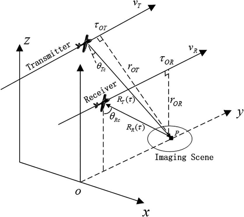
1. Introduction

Bistatic forward-looking synthetic aperture radar (BFSAR) has two platforms installed with a transmitter and receiver, respectively. Despite the separation of the two platforms, the BFSAR can still achieve a high azimuth resolution if a forward-looking geometry is used. Forward-looking imaging is highly desirable in some applications, but it has been a blind sector for monostatic synthetic aperture radar (SAR)¹^–³ for a long time. Therefore, BFSAR has recently received considerable attention.

The peculiarity and feasibility of BFSAR was studied in detail.⁴^–⁶ Through the exploration of the limitation and potential of BFSAR, the best forward-looking geometry was proposed for achieving a high-resolution image. Moreover, some BFSAR experiments were carried out and the exciting imaging results were obtained.⁷^–¹⁰ However, we can find that the imaging algorithms used in these experiments are mostly backprojection algorithms (time-domain algorithms). The time-domain algorithm can work well in arbitrary flight trajectories and no approximation is taken. However, it has a high computational cost and is not available for real-time imaging applications. Therefore, it is urgent to develop new frequency-domain imaging algorithms. Some theories of imaging algorithms for BFSAR have been reported. Based on the extended Loffeld’s bistatic formula (ELBF) method,¹¹ a range-Doppler algorithm is developed.¹² But the ELBF method has its limitations in representing the bistatic point target reference spectrum (BPTRS). A chirp scaling algorithm (CSA) based on the method of Legendre polynomial extension was also proposed.¹³ The accuracy of this imaging solution is decided by the reserved order of an expending Taylor series. With the keystone transform method, a nonlinear chirp scaling algorithm for one-stationary BFSAR was derived.¹⁴ In addition, a modified Omega-k algorithm was also reported.¹⁵

To develop new frequency-domain imaging algorithms, we have to obtain the BPTRS of BFSAR first. The BPTRS derived by the method of series reversion (MSR)¹⁶ has a good focusing performance for the general bistatic configuration, even for extreme squint cases. Due to the series form, it is not easy for MSR to be used for imaging algorithm deduction, especially for chirp scaling and Omega-k algorithms.¹⁷ The Loffeld’s bistatic formula (LBF) was first introduced in Ref. 18. In LBF, the contributions of the transmitter and receiver to the total Doppler frequency are assumed to be the same. This assumption results in the failure of LBF in the extreme configuration (i.e., spaceborne/airborne configuration). The ELBF¹¹ was proposed, but it cannot handle the large squint cases of bistatic SAR. The zeroth-order ELBF¹⁹ obtained two gradient equations to solve the Doppler contributions. However, the method would lead to some degradation when it is used in cases with extreme squint or with forward-looking cases to some extent.¹⁷

In this paper, a modified Loffeld’s bistatic formula (MLBF) has been proposed. Compared to LBF¹⁸ and ELBF,¹¹ it can precisely represent the bistatic point target reference spectrum of bistatic forward-looking SAR. Then, a CSA based on BPTRS was derived. Because CSA is free of interpolation, this algorithm has an obvious superiority in efficiency. Finally, numerical simulations were carried out to validate the focusing solution for BFSAR.

2. Modified Loffeld’s Bistatic Formula

The geometry configuration of BFSAR is shown in Fig. 1. The transmitter works in the side-looking mode and the receiver works in the forward-looking mode, respectively. The two platforms move along the $y$ axis. The mathematical symbols and their definitions used in Fig. 1 are given as follows:

$t$ and $τ$ : Time variables of range and azimuth.
$τ_{OT}$ and $τ_{OR}$ : Zero Doppler times of the transmitter and receiver.
$r_{OT}$ and $r_{OR}$ : The closest ranges from transmitter and receiver to the point target P.
$R_{T} (τ)$ and $R_{R} (τ)$ : Instantaneous slant ranges from the transmitter and receiver to the point target P.
$θ_{T c}$ and $θ_{R c}$ : The squint angle of the transmitter and the forward-looking angle of the receiver at the composite beam center crossing time.
$v_{T}$ and $v_{R}$ : Velocities of the transmitter and receiver, respectively.

Fig. 1

The geometry of bistatic forward-looking synthetic aperture radar (SAR).

The instantaneous slant ranges from the transmitter and receiver to the point target P at time $τ$ are defined as

Eq. (1)

R_{T} (τ) = \sqrt{r_{OT}^{2} + {(τ - τ_{OT})}^{2} v_{T}^{2}},

Eq. (2)

R_{R} (τ) = \sqrt{r_{OR}^{2} + {(τ - τ_{OR})}^{2} v_{R}^{2}} .

Hence, the echo data from target P after demodulation are

Eq. (3)

g (t, τ) = σ_{p} w_{r} [t - \frac{R_{T} (τ) + R_{R} (τ)}{c}] w_{a} (τ - τ_{c}) \exp {j π k_{r} {[t - \frac{R_{T} (τ) + R_{R} (τ)}{c}]}^{2}} \cdot \exp [- j 2 π \frac{R_{T} (τ) + R_{R} (τ)}{λ}],

where

w_{r} (\cdot)

and

w_{a} (\cdot)

are window functions for range and azimuth, respectively;

σ_{p}

is the backscattering coefficient of the point target P;

τ_{c}

is the central azimuth time of the composite azimuth antenna pattern;

c

is the velocity of light;

f_{0}

and

λ

are the carrier frequency and wavelength; and

k_{r}

is the frequency modulated rate of linear frequency modulation signal.

Taking a two-dimensional FFT for Eq. (3), we get

Eq. (4)

g (f, f_{τ}) = σ_{p} w_{r} (f) \exp {- j π \frac{f^{2}}{k_{r}}} \int w_{a} (τ - τ_{c}) \exp [- j ϕ_{b} (f, τ)] d τ,

where

f

and

f_{τ}

represent the range and azimuth frequency variables; the bistatic phase

ϕ_{b} (f, τ)

is given as follows:

Eq. (5)

ϕ_{b} (f, τ) = 2 π (f + f_{0}) \frac{R_{T} (τ) + R_{R} (τ)}{c} + 2 π f_{τ} τ = \frac{2 π (f + f_{0})}{c} [\sqrt{r_{OT}^{2} + {(τ - τ_{OT})}^{2} v_{T}^{2}} + \sqrt{r_{OR}^{2} + {(τ - τ_{OR})}^{2} v_{R}^{2}}] + 2 π f_{τ} τ .

From Eqs. (4) and (5), we can see that the bistatic phase term $ϕ_{b} (f, τ)$ contains a double square root and is included in the integral. It is difficult to obtain the BPTRS from Eq. (4) by directly applying the stationary phase.²⁰^,²¹ Thus, we split the bistatic phase term, Eq. (5), into two components as follows:

Eq. (6)

ϕ_{b} (f, τ) = ϕ_{T} (f, τ) + ϕ_{R} (f, τ),

Eq. (7)

ϕ_{T} (f, τ) = 2 π [\frac{(f + f_{0})}{c} R_{T} (τ) + f_{τ T} τ],

Eq. (8)

ϕ_{R} (f, τ) = 2 π [\frac{(f + f_{0})}{c} R_{R} (τ) + f_{τ R} τ],

where

ϕ_{T} (f, τ)

and

ϕ_{R} (f, τ)

are the phase terms contributed by the transmitter and receiver, respectively.

f_{τ T}

and

f_{τ R}

represent the instantaneous azimuth frequencies for the transmitter and receiver, respectively. In the LBF method,¹⁸ it is assumed that the contributions of the transmitter and receiver to the azimuth modulation are the same. The assumptions are shown as follows:

Eq. (9)

f_{τ T} = f_{τ R} = \frac{f_{τ}}{2} .

However, the real azimuth modulations of the transmitter and receiver are not equal at all when the LBF is used in the extreme configuration (i.e., spaceborne/airborne configuration). Then, ELBF¹¹ formulates $f_{τ T}$ and $f_{τ R}$ as follows:

Eq. (10)

f_{τ T} = k_{T} f_{τ},

Eq. (11)

f_{τ R} = k_{R} f_{τ},

where

k_{T}

and

k_{R}

are the weighting factors, which are defined as the ratio of the time-bandwidth product (TBP) of transmitter and receiver to the total TBP. However, the ELBF shows a limitation in the high squint cases of bistatic SAR since the effect of squint angles on the instantaneous Doppler frequency is neglected.

The zeroth-order ELBF method¹⁹ makes the result of Eq. (12) as small as possible.

Eq. (12)

{‖ E ‖}^{2} = {(τ - τ_{T})}^{2} + {(τ - τ_{R})}^{2},

where

τ_{T}

and

τ_{R}

are the transmitting and receiving points of stationary phases (PSPs). The variables

f_{τ T}

and

f_{τ R}

are included in

τ_{T}

and

τ_{R}

, respectively. This equation does not have an analytical solution, and an approximate solution can be found by using the least square method. The main idea of zeroth-order ELBF is to approximate the difference between the transmitting and receiving PSPs to zero. However, in this method, only the contributions of zeroth-order Doppler frequencies are considered. This would lead to some degradation when the method is used in forward-looking cases with large forward-looking angles.

In this paper, we try to solve the instantaneous azimuth frequencies $f_{τ T}$ and $f_{τ R}$ directly. Here, we redraw the geometries of the flight tracks of the transmitter and receiver, as shown in Fig. 2.

Fig. 2

The flight geometry of transmitter and receiver. (a) The geometry of transmitter’s track. (b) The geometry of receiver’s track.

In Fig. 2, $θ_{T}$ and $θ_{R}$ are the instantaneous squint and forward-looking angles at time $τ$ ; $R_{T c}$ and $R_{R c}$ are the slant ranges of the transmitter and receiver at the composite beam center crossing time $τ_{c}$ . Suppose the transmitter and receiver both start flying at time $τ_{c}$ ; after time $Δ τ$ we can get the following relationship:

Eq. (13)

\frac{R_{T c} \sin θ_{T c} - R_{T c} \cos θ_{T c} \tan θ_{T}}{v_{T}} = \frac{R_{R c} \sin θ_{R c} - R_{R c} \cos θ_{R c} \tan θ_{R}}{v_{R}} .

Meanwhile, the two instantaneous Doppler frequencies satisfy the following relationship:

Eq. (14)

f_{τ} = \frac{f + f_{0}}{c} (v_{T} \sin θ_{T} + v_{R} \sin θ_{R}) = f_{τ T} + f_{τ R} .

Solving the equations composed by Eqs. (13) and (14), we can get the analytic expression of the frequencies $f_{τ T}$ and $f_{τ R}$ . We expand $f_{τ T}$ and $f_{τ R}$ in their Taylor series as follows:

Eq. (15)

{\begin{matrix} f_{τ T} = f_{τ T C} + A_{T 1} (f_{τ} - f_{τ C}) + A_{T 2} {(f_{τ} - f_{τ C})}^{2} + A_{T 3} {(f_{τ} - f_{τ C})}^{3} \\ f_{τ R} = f_{τ R C} + A_{R 1} (f_{τ} - f_{τ C}) + A_{R 2} {(f_{τ} - f_{τ C})}^{2} + A_{R 3} {(f_{τ} - f_{τ C})}^{3} \end{matrix},

where

Eq. (16)

{\begin{cases} f_{τ C} = f_{τ T C} + f_{τ R C} \\ f_{τ T C} = (f_{τ} + f_{c}) v_{T} \sin θ_{T c} / c \\ f_{τ R C} = (f_{τ} + f_{c}) v_{R} \sin θ_{R c} / c \end{cases} .

Combined with Eqs. (13) and (14), coefficients $A_{T 1} \dots A_{T 3}$ , $A_{R 1} \dots A_{R 3}$ can be obtained, then we get the analytic expressions of the frequencies $f_{τ T}$ and $f_{τ R}$ . Although the results in Eq. (15) are more precise than those in Ref. 19 due to the high-order term in Eq. (15), the complexity of the method is greatly increased. It would make present difficulties when we derive the chirp scaling algorithm later. Therefore, some linear approximations are used here to solve Eqs. (13) and (14). We expand $\tan θ_{T}$ and $\tan θ_{R}$ in their Taylor series at $\sin θ_{T} = \sin θ_{T c}$ and $\sin θ_{R} = \sin θ_{R c}$ , respectively, and only reserve the first-order term.

Eq. (17)

{\begin{matrix} \tan θ_{T} = \tan θ_{T c} + \frac{\sin θ_{T} - \sin θ_{T c}}{\cos^{3} θ_{T c}} \\ \tan θ_{R} = \tan θ_{R c} + \frac{\sin θ_{R} - \sin θ_{R c}}{\cos^{3} θ_{R c}} \end{matrix} .

Substituting Eq. (17) into Eq. (13) and combining Eq. (14), the equations are solved as follows:

Eq. (18)

{\begin{matrix} \begin{array}{l} f_{τ T} (f, f_{τ}) = \frac{R_{R c} v_{T}^{2} \cos^{2} θ_{T c} f_{τ}}{R_{T c} v_{R}^{2} \cos^{2} θ_{R c} + R_{R c} v_{T}^{2} \cos^{2} θ_{T c}} \\ \begin{matrix} + \frac{v_{T} (f + f_{0}) (R_{T c} v_{R}^{2} \cos^{2} θ_{R c} \sin θ_{T c} - R_{R c} v_{T} v_{R} \cos^{2} θ_{T c} \sin θ_{R c})}{c (R_{T c} v_{R}^{2} \cos^{2} θ_{R c} + R_{R c} v_{T}^{2} \cos^{2} θ_{T c})} \end{matrix} \end{array} \\ \begin{array}{l} f_{τ R} (f, f_{τ}) = \frac{R_{T c} v_{R}^{2} \cos^{2} θ_{R c} f_{τ}}{R_{T c} v_{R}^{2} \cos^{2} θ_{R c} + R_{R c} v_{T}^{2} \cos^{2} θ_{T c}} \\ \begin{matrix} + \frac{v_{R} (f + f_{0}) (R_{R c} v_{T}^{2} \cos^{2} θ_{T c} \sin θ_{R c} - R_{T c} v_{T} v_{R} \cos^{2} θ_{R c} \sin θ_{T c})}{c (R_{T c} v_{R}^{2} \cos^{2} θ_{R c} + R_{R c} v_{T}^{2} \cos^{2} θ_{T c})} \end{matrix} \end{array} \end{matrix} .

Although linear approximation is used, the max error made by this approximation (with Table 1 simulation parameters, which is discussed later in this paper, the forward-looking angle of the receiver is 45 deg) is $1.85 \times 10^{- 3} rad$ . Therefore, the error can be ignored and Eq. (18) can precisely present the contributions of the transmitter and receiver to the total azimuth modulation. After obtaining the instantaneous azimuth frequency of the transmitter and receiver, we expand Eqs. (7) and (8) at their points of the stationary phase $τ_{T}$ and $τ_{R}$ . The expanded series are truncated at the second-order term, given as

Eq. (19)

ϕ_{T} (τ) \approx ϕ_{T} (τ_{T}) + \frac{1}{2} ϕ_{T}^{''} (τ_{T}) {(τ - τ_{T})}^{2},

Eq. (20)

ϕ_{R} (τ) \approx ϕ_{R} (τ_{R}) + \frac{1}{2} ϕ_{R}^{''} (τ_{R}) {(τ - τ_{R})}^{2},

where

Eq. (21)

τ_{T} = τ_{OT} - \frac{c r_{OT} f_{τ T}}{v_{T}^{2} F_{T}} τ_{R} = τ_{OR} - \frac{c r_{OR} f_{τ R}}{v_{R}^{2} F_{R}},

Eq. (22)

F_{T} = \sqrt{{(f + f_{0})}^{2} - {(\frac{c f_{τ T}}{v_{T}})}^{2}} F_{R} = \sqrt{{(f + f_{0})}^{2} - {(\frac{c f_{τ R}}{v_{R}})}^{2}},

Eq. (23)

ϕ_{T}^{''} (τ_{T}) = \frac{2 π}{c} \frac{v_{T}^{2} F_{T}^{3}}{r_{OT} {(f + f_{0})}^{2}} ϕ_{R}^{''} (τ_{R}) = \frac{2 π}{c} \frac{v_{R}^{2} F_{R}^{3}}{r_{OR} {(f + f_{0})}^{2}} .

Table 1

System parameters in parallel tracks.

Parameters	Transmitter	Receiver
Carrier frequency	9.65 GHz
Range bandwidth	100 MHz
Velocity	$200 m / s$
Pulse recurrence frequency sampling rate	600 Hz 180 MHz
Position	(0,4,8) km	(10,0,4) km
Squint angle	0 deg	/
Forward-looking angle	/	45 deg

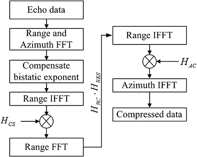
Substituting Eqs. (6), (19), and (20) into Eq. (4), we get

Eq. (24)

g (f, f_{τ}) = σ_{p} w_{r} (f) \exp {- j π \frac{f^{2}}{k_{r}}} \exp {- j [ϕ_{T} (f, τ_{T}) + ϕ_{R} (f, τ_{R})]} \cdot \int w_{a} (τ - τ_{c}) \exp {- \frac{j}{2} [ϕ_{T}^{''} (f, τ_{T}) (τ - τ_{T}) + ϕ_{R}^{''} (f, τ_{R}) (τ - τ_{R})]} d τ .

Applying stationary phase techniques to the last exponent in Eq. (24), we get the bistatic stationary phase $τ_{b}$ .

Eq. (25)

τ_{b} = \frac{r_{OT} v_{R}^{2} F_{R}^{3} τ_{OR} + r_{OR} v_{T}^{2} F_{T}^{3} τ_{OT}}{v_{T}^{2} F_{T}^{3} r_{OR} + v_{R}^{2} F_{R}^{3} r_{OT}} - \frac{c r_{OT} r_{OR} (F_{T}^{2} f_{τ T} + F_{R}^{2} f_{τ R})}{v_{T}^{2} F_{T}^{3} r_{OR} + v_{R}^{2} F_{R}^{3} r_{OT}} .

Finally, we get the BPTRS of the BFSAR.

Eq. (26)

g (f, f_{τ}) = σ_{p} \exp {- j π \frac{f^{2}}{k_{r}}} \exp {- j ψ_{QM}} \exp {- \frac{j}{2} ψ_{BD}},

where

Eq. (27)

ψ_{QM} = ϕ_{T} (f, τ_{T}) + ϕ_{R} (f, τ_{R}) = 2 π (f_{τ T} τ_{OT} + f_{τ R} τ_{OR}) + \frac{2 π}{c} (r_{OT} F_{T} + r_{OR} F_{R}),

Eq. (28)

ψ_{BD} = ϕ_{T}^{''} (f, τ_{T}) {(τ_{b} - τ_{T})}^{2} + ϕ_{R}^{''} (f, τ_{R}) {(τ_{b} - τ_{R})}^{2} = \frac{2 π v_{T}^{2} v_{R}^{2} F_{T}^{3} F_{R}^{3}}{c {(f + f_{0})}^{2} (v_{T}^{2} F_{T}^{3} r_{OR} + v_{R}^{2} F_{R}^{3} r_{OT})} \cdot {[(τ_{OT} - τ_{OR}) - \frac{c}{v_{T}^{2} v_{R}^{2} F_{T} F_{R}} (r_{OT} v_{R}^{2} F_{R} f_{τ T} - r_{OR} v_{T}^{2} F_{T} f_{τ R})]}^{2} .

$ψ_{QM}$ can be considered as the quasi-monostatic phase term, and $ψ_{BD}$ is defined as the bistatic deformation phase term. Before implementing an imaging algorithm, the bistatic deformation phase term should be compensated. The method proposed above can be considered as an MLBF.

3. CSA for the Bistatic Forward-Looking SAR Processing

Instead of interpolation, chirp phase multiplication is used in CSA to correct the range cell migration (RCM). It is an efficient algorithm. However, due to the unknown scaling factor, it is complex to derive CSA based on the BPTRS obtained by the MLBF.

After compensating the bistatic deformation phase term, we transform Eq. (26) into a range-Doppler domain and obtain the expression as

Eq. (29)

g (t, f_{τ}) = σ_{p} \exp [- j \frac{2 π}{c} (r_{OT} D_{T} + r_{OR} D_{R}) f_{0}] \exp [- j 2 π (B \cdot τ_{OT} + E \cdot τ_{OR}) f_{0}] \cdot \exp [- j 2 π (A \cdot τ_{OT} + D \cdot τ_{OR}) f_{τ}] \exp {j π k_{m} {[t - \frac{R (f_{τ})}{c}]}^{2}},

where

Eq. (30)

A = \frac{R_{R c} v_{T}^{2} \cos^{2} θ_{T c}}{R_{T c} v_{R}^{2} \cos^{2} θ_{R c} + R_{R c} v_{T}^{2} \cos^{2} θ_{T c}},

Eq. (31)

B = \frac{v_{T} (R_{T c} v_{R}^{2} \cos^{2} θ_{R c} \sin θ_{T c} - R_{R c} v_{T} v_{R} \cos^{2} θ_{T c} \sin θ_{R c})}{c (R_{T c} v_{R}^{2} \cos^{2} θ_{R c} + R_{R c} v_{T}^{2} \cos^{2} θ_{T c})},

Eq. (32)

D = \frac{R_{T c} v_{R}^{2} \cos^{2} θ_{R c}}{R_{T c} v_{R}^{2} \cos^{2} θ_{R c} + R_{R c} v_{T}^{2} \cos^{2} θ_{T c}},

Eq. (33)

E = \frac{v_{R} (R_{R c} v_{T}^{2} \cos^{2} θ_{T c} \sin θ_{R c} - R_{T c} v_{T} v_{R} \cos^{2} θ_{R c} \sin θ_{T c})}{c (R_{T c} v_{R}^{2} \cos^{2} θ_{R c} + R_{R c} v_{T}^{2} \cos^{2} θ_{T c})},

Eq. (34)

μ_{T 1} = A \cdot \frac{c f_{τ}}{f_{0} v_{T}} + B \cdot \frac{c}{v_{T}} μ_{T 2} = B \cdot \frac{c}{v_{T}},

Eq. (35)

μ_{R 1} = D \cdot \frac{c f_{τ}}{f_{0} v_{R}} + E \cdot \frac{c}{v_{R}} μ_{R 2} = E \cdot \frac{c}{v_{R}},

Eq. (36)

D_{T} = \sqrt{1 - μ_{T 1}^{2}} D_{R} = \sqrt{1 - μ_{R 1}^{2}} .

In Eq. (29), the frequency-modulated rate $k_{r}$ in range is changed by the coupling of the range and azimuth, and the new chirp rate $k_{m}$ in range-Doppler domain is given as

Eq. (37)

k_{m} = \frac{k_{r}}{1 - \frac{c k_{r} f_{τ}^{2}}{f_{0}^{3}} (\frac{A^{2} r_{OT}}{D_{T}^{3} v_{T}^{2}} + \frac{D^{2} r_{OR}}{D_{R}^{3} v_{R}^{2}})} .

In Eq. (29), $R (f_{τ})$ is the range migration of a target and is defined as

Eq. (38)

R (f_{τ}) = c \cdot (B \cdot τ_{OT} + E \cdot τ_{OR}) + \frac{(1 - μ_{T 1} μ_{T 2}) r_{OT}}{D_{T}} + \frac{(1 - μ_{R 1} μ_{R 2}) r_{OR}}{D_{R}} .

We assume the range chirp scaling function for the BFSAR as follows:

Eq. (39)

H_{C S} = \exp {j π k_{m} C_{s} {[t - \frac{R_{ref} (f_{τ})}{c}]}^{2}},

where

C_{s}

is the unknown scaling factor.

R_{ref} (f_{τ})

is the range migration of the reference target, given as

Eq. (40)

R_{ref} (f_{τ}) = c \cdot (B \cdot τ_{OT} + E \cdot τ_{OR}) + \frac{(1 - μ_{T 1} μ_{T 2}) r_{OT_ref}}{D_{T}} + \frac{(1 - μ_{R 1} μ_{R 2}) r_{OR_ref}}{D_{R}} .

In Ref (41), $r_{OT_ref}$ and $r_{OR_ref}$ are the closest ranges from the transmitter and receiver to the reference target. (The target located at the middle of the imaging scene is usually chosen as the reference target.) We multiply Eq. (29) by Eq. (39) and implement FFT in the range direction, and then get

Eq. (41)

G_{1} (f, f_{τ}) = σ_{p} \exp [- j \frac{2 π}{c} (r_{OT} D_{T} + r_{OR} D_{R}) f_{0}] \exp [- j 2 π (B \cdot τ_{OT} + E \cdot τ_{OR}) f_{0}] \cdot \exp [- j 2 π (A \cdot τ_{OT} + D \cdot τ_{OR}) f_{τ}] \exp [- j π \frac{f^{2}}{(1 + C_{s}) k_{m}}] \cdot \exp [- j 2 π f \frac{R (f_{τ}) + C_{s} R_{ref} (f_{τ})}{(1 + C_{s}) c}] \exp {j π k_{m} \frac{C_{s} {[R (f_{τ}) - R_{ref} (f_{τ})]}^{2}}{(1 + C_{s}) c^{2}}} .

In Eq. (41), we can clearly see that the total RCM is

Eq. (42)

RCM = \frac{R (f_{τ}) + C_{s} R_{ref} (f_{τ})}{1 + C_{s}} .

Because the translational invariant case is used in this paper, we make some linear approximations.¹² The approximations are given as

Eq. (43)

τ_{O T} = p_{0} + τ_{O R},

Eq. (44)

r_{OT} = p_{1} + p_{2} r_{OR},

where

p_{0}

,

p_{1}

, and

p_{2}

are all coefficient factors. Therefore, we can transform the total RCM as follows:

Eq. (45)

RCM = c [B \cdot p_{0} + (B + E) τ_{OR}] + \frac{(1 - μ_{T 1} μ_{T 2}) p_{1}}{D_{T}} + \frac{C_{s} r_{OR_ref}}{1 + C_{s}} [\frac{(1 - μ_{T 1} μ_{T 2}) p_{2}}{D_{T}} + \frac{1 - μ_{R 1} μ_{R 2}}{D_{R}}] + \frac{r_{OR}}{1 + C_{s}} [\frac{(1 - μ_{T 1} μ_{T 2}) p_{2}}{D_{T}} + \frac{1 - μ_{R 1} μ_{R 2}}{D_{R}}],

where the last term of the RCM is a range variant term. In order to remove the range variant of the total RCM on the Doppler frequency, we let

Eq. (46)

\frac{r_{OR}}{1 + C_{s}} [\frac{(1 - μ_{T 1} μ_{T 2}) p_{2}}{D_{T}} + \frac{1 - μ_{R 1} μ_{R 2}}{D_{R}}] = (1 + p_{2}) r_{OR} .

Then, the analytic formula of the scaling factor

C_{s}

is obtained as

Eq. (47)

C_{s} = \frac{1}{1 + p_{2}} [\frac{(1 - μ_{T 1} μ_{T 2}) p_{2}}{D_{T}} + \frac{1 - μ_{R 1} μ_{R 2}}{D_{R}}] - 1 .

Therefore, after substituting Eq. (47) into Eq. (41), we can rewrite Eq. (41) without unknown variables. Then, we use the following matching filters to complete the image focusing:

Eq. (48)

H_{RC} = \exp [j π \frac{f^{2}}{(1 + C_{s}) k_{m}}] \cdot \exp {j \frac{2 π C_{s} r_{OR_ref}}{c (1 + C_{s})} [\frac{(1 - μ_{T 1} μ_{T 2}) p_{2}}{D_{T}} + \frac{1 - μ_{R 1} μ_{R 2}}{D_{R}}] f},

Eq. (49)

H_{RES} = \exp {- j π k_{m} \frac{C_{s} {[R (f_{τ}) - R_{ref} (f_{τ})]}^{2}}{(1 + C_{s}) c^{2}}},

Eq. (50)

H_{AC} = \exp [j 2 π (A \cdot τ_{OT} + D \cdot τ_{OR}) f_{τ}] \exp [j \frac{2 π}{c} (r_{OT} D_{T} + r_{OR} D_{R}) f_{0}] \cdot \exp [j 2 π (B \cdot τ_{OT} + E \cdot τ_{OR}) f_{0}],

where

H_{RC}

is used for range compression (RC), the second range compression, and the bulk range cell migration correction;

H_{AC}

is used for azimuth compression; and

H_{RES}

is used to remove the residual phase term introduced by the chirp scaling multiplication. The corresponding block diagram of the CSA for the BFSAR is shown in Fig. 3.

Fig. 3

Block diagram of chirp scaling algorithm (CSA) used in bistatic forward-looking SAR.

4. Simulation Results

In order to verify the focusing solution for the BFSAR, two simulation experiments are carried out in this section. The first experiment is to determine whether the BPTRS obtained by the MLBF is appropriate for the BFSAR case and to simultaneously compare the performance of the MLBF with those of other proposed methods. The second experiment is to validate the effectiveness of the proposed CSA.

The simulation parameters are listed in Table 1. We use the analytical BPTRS to focus the BPTRS obtained by LBF,¹⁸ ELBF,¹¹ MLBF, and the spectra derived from the MSR using the fourth-order expansion.¹⁶ The focusing results are shown in Fig. 4.

Fig. 4

Focusing results. (a) Processing result using Loffeld’s bistatic formula (LBF). (b) Processing result using extended LBF. (c) Processing result using modified LBF (MLBF). (d) Processing result using method of series reversion. (e) Comparison results of the azimuth profiles obtained from Figs. 4(c) and 4(d).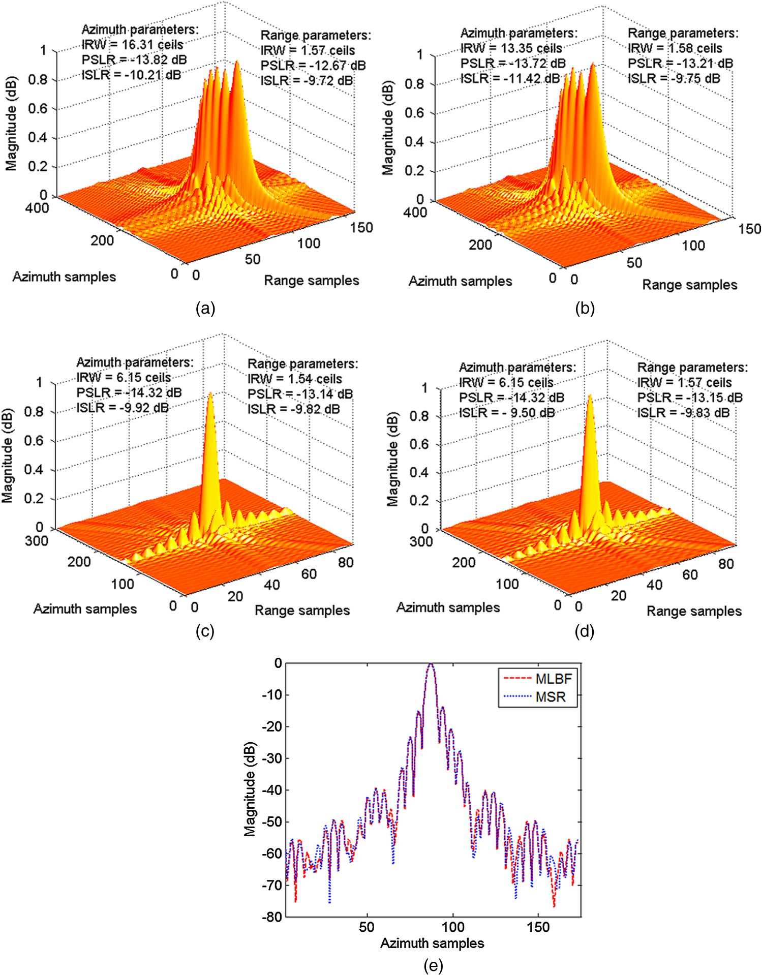

From Figs. 4(a) and 4(b), we can see that the LBF and ELBF have severe degradation in the azimuth direction. They are not appropriate for bistatic forward-looking SAR cases. In general, the LBF method and ELBF method reach their limit when the forward-looking angle is 30 and 40 deg, respectively. Figures 4(c) and 4(d) reveal that MLBF and MSR are all focused on the point target. Furthermore, Fig. 4(e) shows the azimuth profiles of the MLBF and MSR. It is clear that the method proposed in this paper agrees with the MSR. However, the resulting accuracy of the spectrum from the MSR is dependent on the number of terms in the expansion. Here, we use the fourth-order expansion of the MSR. However, the spectrum of the MLBF is a closed form with a second term and still has a good performance. In addition, it is not easy for the MSR to be used for imaging algorithm deduction.

The CSA imaging results are shown in Fig. 5.

Fig. 5

CSA imaging results based on the bistatic point target reference spectrum obtained by MLBF. (a) The locations of simulated targets. (b) The contours of final imaging result with 30 dB dynamic range. (c) The azimuth profile of the target P9. (d) The range profile of the target P9.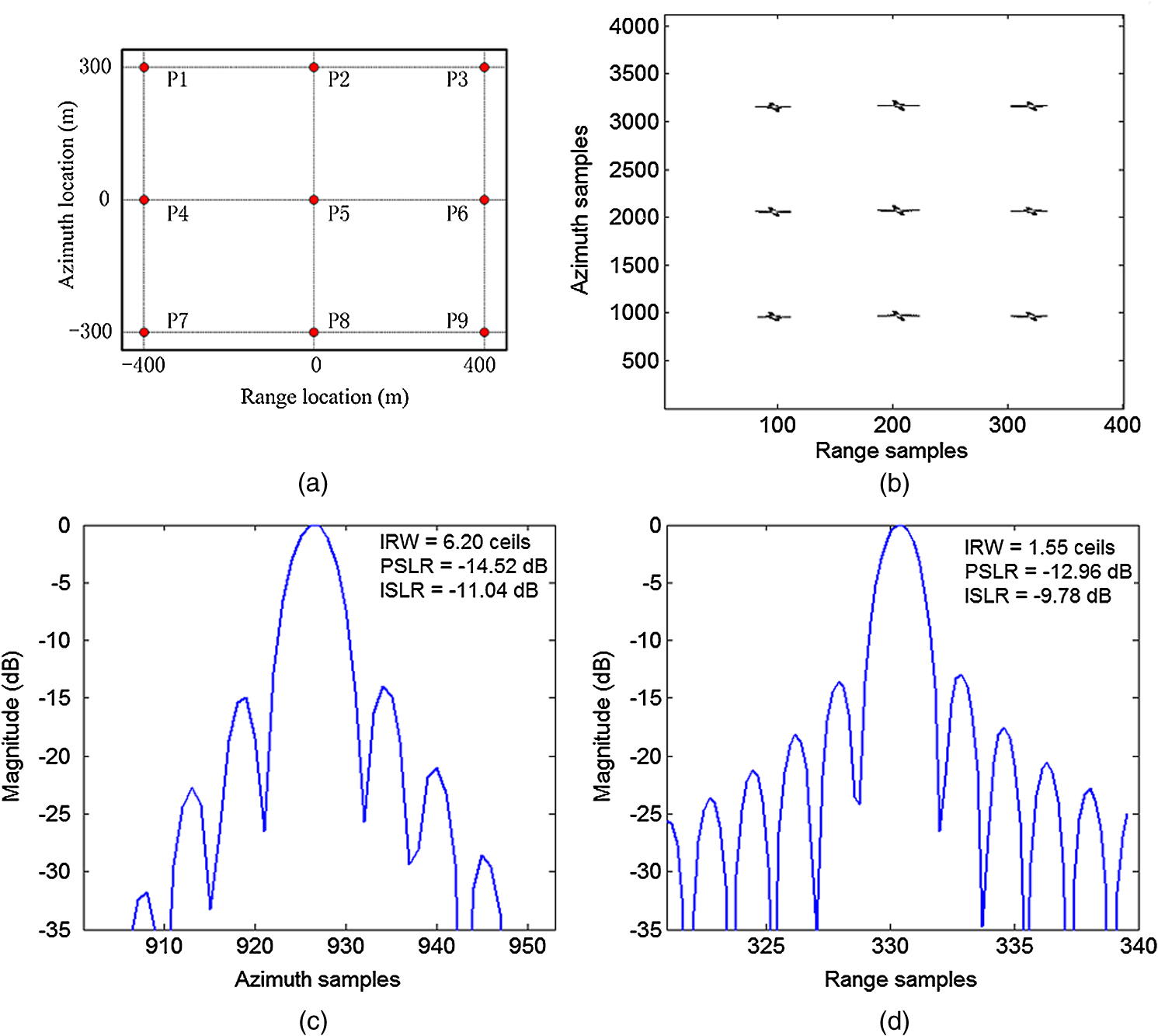

Figure 5(a) shows the locations of the simulated targets, where the distances between two adjacent targets along the range and azimuth directions are, respectively, 400 and 300 m. Figure 5(b) represents the contours of the final imaging result. The dynamic range shown in this picture is 30 dB. In order to further evaluate the imaging quality, Figs. 5(c) and 5(d) present the impulse profiles of the target P9 in the azimuth and range directions, respectively. The peak sidelobe ratio (PSLR) of the azimuth profile is $- 14.52 dB$ , and the integrated sidelobe ratio (ISLR) is $- 11.04 dB$ . The PSLR of the range profile is $- 12.96 dB$ , and the ISLR is $- 9.78 dB$ . More image quality parameters are listed in Table 2. The ideal impulse response width (IRWs) of the azimuth and range are 6.04 and 1.52 ceils (or samples), respectively. We can find that all the targets are well focused.

Table 2

Image quality parameters.

Targets	Range			Azimuth
Targets	PSLR (dB)	ISLR (dB)	IRW (ceils)	PSLR (dB)	ISLR (dB)	IRW (ceils)
PT1	$- 12.96$	$- 9.77$	1.54	$- 14.42$	$- 10.96$	6.14
PT5	$- 13.02$	$- 9.80$	1.54	$- 14.53$	$- 11.10$	6.06
PT9	$- 12.96$	$- 9.78$	1.55	$- 14.52$	$- 11.04$	6.20

PSLR, peak sidelobe ratio; ISLR, integrated sidelobe ratio.

5. Conclusions

A focusing solution for bistatic forward-looking SAR was presented in this paper. First, an MLBF was proposed to obtain the BPTRS. Then, a chirp scaling algorithm based on the BPTRS was derived. Compared to other imaging algorithms, CSA is free of interpolation. Finally, two simulation experiments were carried out to validate the focusing solution. The simulation results showed that the BPTRS obtained by the MLBF was more precise than the LBF and ELBF, and that the focusing capability of the derived CSA is high.

Acknowledgments

This paper is supported by the PhD programs foundation of Ministry of China (Grant No. 20113219110018), the Ministry Pre-research Foundation (Grant No. 9140A07010713BQ02025), National Natural Science Foundation of China (Grant No. 61302188), and Natural Science Foundation of Jiangsu Province (Grant No. BK20131005).

References

1.

O. DoganM. Kartal, “Efficient stripmap-mode SAR raw data simulation including platform angular deviations,” IEEE Geosci. Remote Sens. Lett., 8 (4), 784 –788 (2011). http://dx.doi.org/10.1109/LGRS.2011.2112633 IGRSBY 1545-598X Google Scholar

2.

S. H. ShimY. M. Ro, “Practical synthetic aperture radar image formation based on realistic spaceborne synthetic aperture radar modeling and simulation,” J. Appl. Remote Sens., 7 (1), 073494 (2013). http://dx.doi.org/10.1117/1.JRS.7.073494 1931-3195 Google Scholar

3.

Q. Q. PengL. Zhao, “Novel mixture model for synthetic aperture radar imagery,” J. Appl. Remote Sens., 6 (1), 063616 (2012). http://dx.doi.org/10.1117/1.JRS.6.063616 1931-3195 Google Scholar

4.

J. BalkeD. MatthesT. Mathy, “Illumination constraints for forward-looking radar receivers in bistatic SAR geometries,” in European Radar Conf., 25 –28 (2008). Google Scholar

5.

J. Wuet al., “Bistatic forward-looking SAR: theory and challenges,” in IEEE Radar Conf., 1 –4 (2009). Google Scholar

6.

I. Walterscheidet al., “Potential and limitations of forward-looking bistatic SAR,” in IEEE Int. Geoscience and Remote Sensing Symp., 216 –219 (2010). Google Scholar

7.

J. Wuet al., “First result of bistatic forward-looking SAR with stationary transmitter,” in IEEE Int. Geoscience and Remote Sensing Symp., 1223 –1226 (2011). Google Scholar

8.

T. Espeteret al., “Bistatic forward-looking SAR experiments using an airborne receiver,” in Proc. Int. Radar Symp., 41 –46 (2011). Google Scholar

9.

J. Balke, “SAR image formation for forward-looking radar receivers in bistatic geometry by airborne illumination,” in IEEE Radar Conf., 1 –5 (2008). Google Scholar

10.

I. Walterscheidet al., “Bistatic spaceborne-airborne forward-looking SAR,” in 8th European Conf. on Synthetic Aperture Radar, 1 –4 (2010). Google Scholar

11.

R. Wanget al., “A bistatic point target reference spectrum for general bistatic SAR processing,” IEEE Geosci. Remote Sens. Lett., 5 (3), 517 –521 (2008). http://dx.doi.org/10.1109/LGRS.2008.923542 IGRSBY 1545-598X Google Scholar

12.

R. Wanget al., “Image formation algorithm for bistatic forward-looking SAR,” in IEEE Int. Geoscience and Remote Sensing Symp., 4091 –4094 (2010). Google Scholar

13.

J. Wuet al., “Focusing bistatic forward-looking SAR using chirp scaling algorithm,” in IEEE Radar Conf., 1036 –1039 (2011). Google Scholar

14.

J. Wuet al., “Focusing bistatic forward-looking SAR with stationary transmitter based on keystone transform and nonlinear chirp scaling,” IEEE Geosci. Remote Sens. Lett., 11 (1), 148 –152 (2014). http://dx.doi.org/10.1109/LGRS.2013.2250904 IGRSBY 1545-598X Google Scholar

15.

H. S. ShinJ. T. Lim, “Omega-k algorithm for airborne forward-looking bistatic spotlight SAR imaging,” IEEE Geosci. Remote Sens. Lett., 6 (2), 312 –316 (2009). http://dx.doi.org/10.1109/LGRS.2008.2011924 IGRSBY 1545-598X Google Scholar

16.

Y. L. NeoF. WongI. G. Cumming, “A two-dimensional spectrum for bistatic SAR processing using series reversion,” IEEE Geosci. Remote Sens. Lett., 4 (1), 93 –96 (2007). http://dx.doi.org/10.1109/LGRS.2006.885862 IGRSBY 1545-598X Google Scholar

17.

J. Wuet al., “A new look at the point target reference spectrum for bistatic SAR,” Progr. Electromagn. Res., 119 363 –379 (2011). http://dx.doi.org/10.2528/PIER11050704 PELREX 1043-626X Google Scholar

18.

O. Loffeldet al., “Models and useful relations for bistatic SAR processing,” IEEE Trans. Geosci. Remote Sens., 42 (10), 2031 –2038 (2004). http://dx.doi.org/10.1109/TGRS.2004.835295 IGRSD2 0196-2892 Google Scholar

19.

R. Wanget al., “Extending Loffeld’s bistatic formula for general bistatic SAR configuration,” IET Radar Sonar Navig., 4 (1), 74 –84 (2010). http://dx.doi.org/10.1049/iet-rsn.2009.0099 1751-8784 Google Scholar

20.

C. Maet al., “Focusing bistatic forward-looking synthetic aperture radar based on modified hyperbolic approximating,” Acta Physica Sinica, 63 (2), 028403 (2014). http://dx.doi.org/10.7498/aps.63.028403 WLHPAR 1000-3290 Google Scholar

21.

R. Wanget al., “Processing the azimuth-variant bistatic SAR data by using monostatic imaging algorithms based on two-dimensional principle of stationary phase,” IEEE Trans. Geosci. Remote Sens., 49 (10), 3504 –3520 (2011). http://dx.doi.org/10.1109/TGRS.2011.2129573 IGRSD2 0196-2892 Google Scholar

Biography

Chao Ma received his BS degree from Hubei Engineering University, Hubei, China, in 2010. He is currently working toward his PhD degree in information and communication engineering at the Nanjing University of Science and Technology, Jiangsu, China, and is trained in the Institute of Electronic Engineering and Optoelectronic Technology. His research interests include synthetic aperture radar (SAR) signal processing and short-range imaging.

Hong Gu received his MS degree from Nanjing University of Science and Technology, Jiangsu, China, in 1991 and his PhD degree from Xidian University, Shanxi, China, in 1995. He is currently a professor, a Chinese Institute of Electronics senior member, and a member of the radar branch of the Jiangsu Electronic Society. His research interests include noise SAR, radar signal processing and information systems.

Weimin Su received his PhD degree from Nanjing University of Science and Technology, Jiangsu, China, in 1998. He is currently a professor, a senior member of the Chinese Institute of Electronics, a member of the Signal Processing Society of China, and a liaison of Nanjing University of Science and Technology, Jiangsu, China. His research interests include advanced SAR systems and signal processing technology.

Chuanzhong Li received his BS degree from Nanjing University of Science and Technologu, Jiangsu, China, in 2010. He is currently working toward his PhD degree in information and communication engineering at Nanjing University of Science and Technology, Jiangsu, China. His research interests include radar signal processing and noise SAR imaging.

Jinli Chen received his PhD degree from Nanjing University of Science and Technology, Jiangsu, China, in 2010. He is currently working in the Nanjing University of Information Science and Technology as a lecturer. His research interests include multiple input multiple output (MIMO) radar signal processing and high-speed moving target detecting.

CC BY: © The Authors. Published by SPIE under a Creative Commons Attribution 4.0 Unported License. Distribution or reproduction of this work in whole or in part requires full attribution of the original publication, including its DOI.

Citation Download Citation

Chao Ma, Hong Gu, Weimin Su, Chuanzhong Li, and Jinli Chen "Focusing bistatic forward-looking synthetic aperture radar based on modified Loffeld’s bistatic formula and chirp scaling algorithm," Journal of Applied Remote Sensing 8(1), 083586 (22 July 2014). https://doi.org/10.1117/1.JRS.8.083586

Published: 22 July 2014

Access the abstract

JOURNAL ARTICLE
12 PAGES

DOWNLOAD PAPER SAVE TO MY LIBRARY

GET CITATION

CITATIONS

Cited by 2 scholarly publications.

Explore citations on Lens.org

KEYWORDS

Technetium

Synthetic aperture radar

Receivers

Transmitters

Algorithm development

Detection and tracking algorithms

Doppler effect

1.

Introduction

2.

Modified Loffeld’s Bistatic Formula

Fig. 1

Eq. (1)

Eq. (2)

Eq. (3)

Eq. (4)

Eq. (5)

Eq. (6)

Eq. (7)

Eq. (8)

Eq. (9)

Eq. (10)

Eq. (11)

Eq. (12)

Fig. 2

Eq. (13)

Eq. (14)

Eq. (15)

Eq. (16)

Eq. (17)

Eq. (18)

Eq. (19)

Eq. (20)

Eq. (21)

Eq. (22)

Eq. (23)

Table 1

Eq. (24)

Eq. (25)

Eq. (26)

Eq. (27)

Eq. (28)

3.

CSA for the Bistatic Forward-Looking SAR Processing

Eq. (29)

Eq. (30)

Eq. (31)

Eq. (32)

Eq. (33)

Eq. (34)

Eq. (35)

Eq. (36)

Eq. (37)

Eq. (38)

Eq. (39)

Eq. (40)

Eq. (41)

Eq. (42)

Eq. (43)

Eq. (44)

Eq. (45)

Eq. (46)

Eq. (47)

Eq. (48)

Eq. (49)

Eq. (50)

Fig. 3

4.

Simulation Results

Fig. 4

Fig. 5

Table 2

5.

Conclusions

Acknowledgments

References

Biography

Show All Keywords

Keywords/Phrases

Search In:

Publication Years