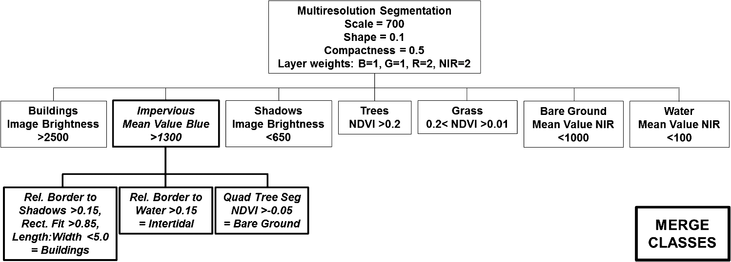
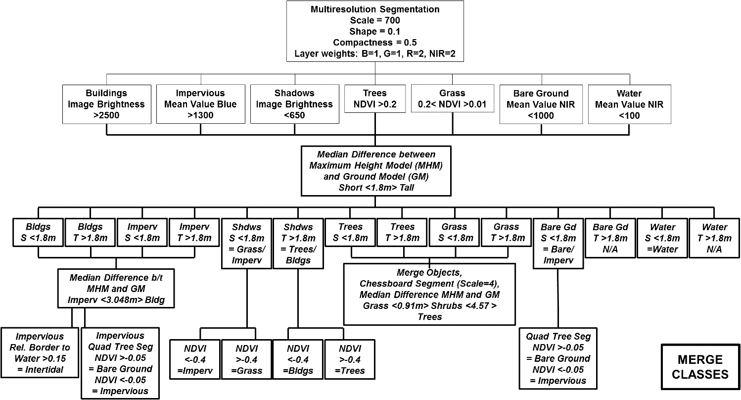
2.1.

Study Area

The study area is a $\sim 6.54\text{-}\mathrm{hectare}$ transect along a rural to urban gradient, located within the city of Olympia, Washington, USA (Fig. 1). The city of Olympia is located at the southern end of Puget Sound and is experiencing a moderate population growth with a population that is expected to double in 30 to 40 years.⁴⁹ Puget Sound provides numerous ecosystem services to the region’s residents and Olympia’s urban tree canopy, detectable through LULC mapping, plays a vital role.

Fig. 1

Map of study area: South Puget Sound, Olympia, Washington, USA.

2.2.

Remote Sensing Datasets

In this work, we used 16-bit, four-band, color infrared imagery acquired in March of 2008 with a pixel resolution of 0.12 m (0.4 feet). On March 2 to 3, 2008 discrete-point LiDAR data were also acquired over the study area with the Optech 3100 sensor at a survey altitude of 899.16 m (2950 feet). Accuracy of the LiDAR data conforms to Puget Sound LiDAR Consortium standards⁵⁰ with an absolute vertical accuracy of 0.03 m RMSE (0.11 feet RMSE). The data point cloud was collected at 4 pulse returns with a density of $4.66\text{first returns}/{\mathrm{m}}^2$. Figure 2 shows the various images representing the remote sensing datasets used in this study.

Fig. 2

Remotely sensed data used to develop the object-based image analysis land use/land cover (LULC) algorithm: (a) false-color near-infrared aerial imagery, (b) LiDAR point cloud colored by true color RGB values, (c) LiDAR data colored by height, (d) LiDAR extruded by height and colored by true color RGB values from the coregistered imagery, and (e) LiDAR point cloud colored by LiDAR height; all scenes show the Washington State Capitol Building.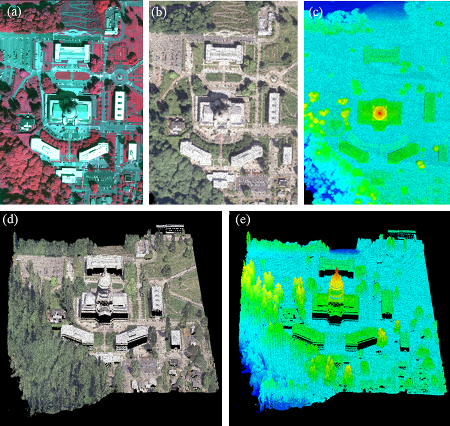

We generated a 1-m per-pixel spatial resolution LiDAR data-based digital terrain model (DTM) using the freely available FUSION software developed by the USDA Forest Service, Pacific Northwest Research Station.^51,52 To accomplish this, we used the groundfilter algorithm within FUSION to filter the likely ground points from the LiDAR point cloud, and then created a smoothed raster from that point cloud at a 1-m resolution. We then applied the ground model to produce the same resolution standardized canopy height metrics which, in conjunction with the ground model, were the key LiDAR-based variables in our OBIA-driven classification.

2.3.

Land Use/Land Cover Classification

2.3.1.

Developing a basic classification

We originally developed an OBIA algorithm for a separate LULC classification project in Seattle, Washington,¹⁴ and wanted see if it would work in different locations within the same ecoregion (i.e., urbanized Pacific Northwest coastal areas) with limited modification. The LULC classes we selected are prominent throughout the greater Pacific Northwest coastal region and although certain classes are under-represented in this specific study area (e.g., intertidal and bare ground), we wanted to keep these classes in the algorithm for future OBIA analyses in different study areas across the Pacific Northwest coast.⁴⁷

Two different LULC classification approaches were used in this study—one approach used imagery alone (IA) while the second used $\mathrm{I}+\mathrm{L}$ data. We used Trimble’s® eCognition® software program to create a segmentation and basic classification for each of the two datasets (IA and $\mathrm{I}+\mathrm{L}$). In both cases, the classification process began with a multiresolution segmentation of the four-band aerial imagery, using a scale parameter of 700, a shape parameter of 0.1, a compactness parameter of 0.5, and layer weights of $\text{blue}=1$, $\text{green}=1$, $\text{red}=2$, and $\text{near-infrared}=2$ (Fig. 3). These specific parameters were selected based on skilled visual interpretation of the image segmentations that resulted from using different scale parameters. Although we do recognize the inherent subjectivity in segmentation scale selection and the resulting image object size, an in-depth discussion on that topic is beyond the scope of our study. Several other published studies have focused on segmentation scale selection optimization and have documented how widely these parameters can vary depending on the object(s) of interest.^53–55

Fig. 3

Decision tree for the initial basic classifications for both imagery alone (IA) and imagery and LiDAR.

We used a combination of logical values, the feature space optimization tool, and two-dimensional (2-D) feature space plots in eCognition®, as well as expert interpretation to select threshold values. LiDAR data thresholds were assigned based on logical height cutoff points for distinguishing between tall and short objects. The mean brightness of each object, computed as the mean of the four bands, was used to classify buildings and shadows at each brightness extreme (i.e., light and dark). Normalized difference vegetation index (NDVI) thresholds were based on logical breakpoints between photosynthetically active tree vegetation, senescent grass, and nonphotosynthetic impervious surfaces. Feature space optimization and 2-D feature space plots allowed us to find appropriate thresholds using brightness for rooftops, darkness for shadows, darkness in the near-infrared for water, darkness in near-infrared for bare ground, and brightness in the blue band for impervious surfaces. Finally, the classification was further improved by implementing several hierarchical rules to remove small misclassified objects enclosed by other objects (e.g., cars on freeways).

2.3.2.

Classification using imagery alone

At the end of the processes described above, we had a basic classification based solely on imagery; however, it contained multiple objects misclassified as shadows, did not discriminate well between buildings and ground impervious surfaces, and misclassified intertidal areas as ground impervious. Several extra rules were written into the algorithm to address these errors (Fig. 4). The rule relative border to shadows ($>0.15$) was used to identify and classify buildings incorrectly assigned to the ground impervious class. This worked well for us because buildings cast shadows, but ground impervious surfaces do not. Next, building shadows were classified by finding the object with the largest classified border, and classifying the shadow by that object’s class. A second rule for buildings was then run based on finding ground impervious objects with a large rectangular fit ($>0.85$) and a small length:width ratio ($<5.0$). This located objects that had a general square shape, and helped to find buildings that did not have large relative borders to shadows (such as those surrounded by trees). Intertidal areas misclassified as ground impervious surfaces were reclassified based on their relative border to water ($>0.15$). Finally, bare ground was located by performing a quad tree segmentation on the ground impervious surfaces layer and classifying objects with an NDVI value greater than $-0.05$ as bare ground. A final set of filtering algorithms filtered out any remaining small misclassified objects.

Fig. 4

Decision tree for the IA classification, including parameter thresholds (additional rules to initial basic classification shown in bold italic).

2.3.3.

Classification using imagery and LiDAR data

We also needed to apply additional rules to an $\mathrm{I}+\mathrm{L}$ classification to compensate for objects classified in error (Fig. 5). The median difference between the maximum height model and the ground model was computed for all objects. This value represented a good approximation of the height of each object above ground, and a threshold of 1.8 m (6 feet) was used to separate tall objects such as buildings and trees, from short objects such as grass and ground impervious surfaces. Shadows were first classified into temporary classes based on median difference. Using an NDVI threshold ($-0.4$) tall temporary objects were classified as trees or buildings, and short temporary objects as grass or ground impervious. A chessboard segmentation was then run on the grass and tree classes, followed by a reclassification based on median height. The median height value was better at explaining differences between these two classes because irrigated lawns created confusion when using NDVI alone. Median height was used to reclassify ground impervious surfaces and buildings. Intertidal areas misclassified as ground impervious were reclassified based on their relative border to water ($>0.15$). As in the IA classification, bare ground was located using a quad tree segmentation and an NDVI threshold ($-0.05$) of the ground impervious class. Lastly, a set of filtering algorithms removed small misclassified objects.

Fig. 5

Decision tree for the $\mathrm{imagery}+\mathrm{LiDAR}$ ($\mathrm{I}+\mathrm{L}$) classification, including parameter thresholds (additional rules to initial basic classification shown in bold italic).

2.4.

Accuracy Assessment

An accuracy assessment was conducted for the four different classifications: IA and $\mathrm{I}+\mathrm{L}$, each with and without postclassification. Accuracy assessment methods were based on the guidelines of Foody^2,56 and Congalton and Green.⁵⁷ First, the area of each class was quantified using polygons from the $\mathrm{I}+\mathrm{L}$ segmentation algorithm (without manual postclassification) for all tiles in study area. These were used to determine the number of points that should fall in each class. Buffering was not used as we did not want to bias our analysis toward large objects which tend to be classified correctly by OBIA methods. We then generated a total of 300 stratified random points, which were distributed proportionally by area for each class, for visual accuracy assessment of the classifications by an expert image analyst. Each point was then visually classified by a trained image analyst using 12 cm color infrared imagery and a canopy/building surface model created using the LiDAR data. The classes used are described in Table 1.

Table 1

Land use/land cover class descriptions.

3.1.

Accuracy for Imagery Alone Classification

The OBIA method produced sufficient results using the aerial IA; overall accuracy was 71.3% ($\mathrm{khat}=0.59$). The method was effective at extracting trees/shrubs, and to a lesser degree, ground impervious surfaces (e.g., roads, driveways, paved parking lots). With the exception of water, tree canopy was classified most effectively, and had a producer’s accuracy of 92.7% and a user’s accuracy of 77.4% ($\mathrm{khat}=0.59$). Since the producer’s accuracy was greater than the user’s accuracy, these results suggest that we have captured the finest amount of detail in our classification these data will allow. This also indicates that the classification algorithm has overclassified tree canopy, and points were generally misclassified as grass. The ground impervious class had a producer’s accuracy of 66% and user’s accuracy of 75.6% ($\mathrm{khat}=0.71$), indicating we may have been able to optimize the algorithm further to achieve a higher producer’s accuracy. Ground impervious surface points were misclassified across all classes except water. Producer’s accuracy for the remaining classes was near or below 50%, excluding water.

3.2.

Accuracy for Imagery Alone Classification with Postclassification

The overall classification accuracy slightly improved to 74.7% ($\mathrm{khat}=0.56$). Again, the method appeared to be effective at extracting tree canopy and ground impervious surfaces. Producer’s accuracy was greater than user’s accuracy for the tree canopy and building classes. Although producer’s accuracy decreased by $<1\%$ for tree/shrubs, there was an increase in producer’s accuracy for the grass class, improving from 36% to 42%. Manual postclassification also increased producer’s accuracy for ground impervious (from 66% to 72.3%), buildings (from 52% to 68%), and water (from 96% to 100%).

3.3.

Accuracy for Imagery and LiDAR Classification

The addition of LiDAR data to the LULC classification process improved the overall classification accuracy to 79.7% ($\mathrm{khat}=0.77$), and enabled us to separate the tree/shrub class into two distinct tree and shrub classes. Interestingly, this method appeared to be more effective at extracting grass and buildings than trees and ground impervious surfaces, as was the case with the IA classification algorithm. The grass class had a producer’s accuracy of 90%, but a user’s accuracy of 64.3%, as some of these points still appear as trees, shrubs, or even bare ground. Producer’s and user’s accuracies for the building class were equal at 88%, and demonstrate the improvement in accuracy the LiDAR data provided for this class. For both tree and ground impervious classes, user’s accuracy was greater than producer’s accuracy, which was 92.7% versus 84.17% and 88.10% versus 78.7%, respectively. Although separated from the tree class, the shrub class had a low producer’s accuracy of 52.9% (user’s accuracy 50%; $\text{khat}=0.47$).

3.4.

Accuracy for Imagery and LiDAR Classification with Postclassification

The small amount of time taken to postclassify the $\mathrm{I}+\mathrm{L}$ classification ($\sim 4\mathrm{h}$) resulted in a 1% improvement of overall classification accuracy from 79.7% to 80.7%. Since the LiDAR data appeared to have cleared up most of the points classified in error on the IA classification, there were fewer points of error in the $\mathrm{I}+\mathrm{L}$ classification. Manual postclassification slightly improved the producer’s accuracy of the ground impervious and water classes from 78.7% and 96% to 83% and 100%, respectively. The manual postclassification also had the benefit of resolving large, obvious errors that comprised a small percentage of the landscape, but were especially glaring when viewing the final map, thus improving the overall quality of the product.

3.5.

Comparisons Between the Four Classifications

As is evident in Table 2, the overall accuracy increased with each classification iteration. Two of our main objectives were to determine the contribution of LiDAR data to classification accuracies and assess the impact of manual postclassification on classification accuracies. Manual postclassification was more time intensive for the IA classification; $\sim 12\mathrm{h}$ of work resulted in a 3.3% increase in overall classification accuracy. Most of this improvement was reflected in increases in the building and ground impervious class accuracies. When LiDAR data were added to the classification, overall accuracy increased an additional 5%. Substantial increases in producer’s accuracy are observed in the grass, building, and ground impervious classes. The addition of LiDAR data enabled us to divide the tree/shrub class into separate tree and shrub classes, which resulted in a higher level of classification detail but lower class accuracies. We assume this is in part due to the confusion between low tree crown edges and actual shrubs, but also to the inability of the image interpreter to determine object height (i.e., trees versus shrubs) on the 2-D imagery used as ground truth. Although producer’s accuracy in the tree class decreased in the $\mathrm{I}+\mathrm{L}$ classifications, user’s accuracy significantly increased.

Table 2

Overall and producer’s accuracies for all four classifications, and percent improvement in accuracies over imagery alone (IA) for each subsequent classification iteration [i.e., IA with postclassification (PC), imagery and LiDAR (I+L, and I+L with PC].

Manual postclassification of the $\mathrm{I}+\mathrm{L}$ classification took $\sim 4\mathrm{h}$ and improved the overall accuracy 1%. The overall difference from the IA classification (without manual postclassification) and the $\mathrm{I}+\mathrm{LiDAR}$ data classification (with manual postclassification) was 9.4%, improving from 71.3% to 80.7% (Table 2). Manual postclassification did not significantly increase the accuracy of our classifications; however, we believe any amount of increase in accuracy is desirable, and based on the short amount of time it takes to do, it is worth the investment. Not only is the accuracy of the map improved but a more visually pleasing product is created as well. For example, in the absence of manual postclassification, we would have shown the State Capitol Building as covered and surrounded by water, which in actuality is merely a shadow cast by the Capitol rotunda (see Fig. 6).

Fig. 6

LULC classifications: (a) IA, (b) IA with postclassification, (c) imagery and LiDAR ($\mathrm{I}+\mathrm{L}$), (d) imagery and LiDAR with postclassification. Notes: (a) and (b) do not contain the shrub class. Misclassification errors in (a) and (b) visually illustrate how the addition of LiDAR can increase class accuracies.

3.6.

Error Attribution

3.7.

Other Issues

Other than those issues described above, the only other error apparent in our $\mathrm{I}+\mathrm{L}$ classification is due to the presence of artifacts at the LiDAR data seams, or tile boundaries (see vertical artifact in Fig. 6). This can be resolved by a few different tiling and stitching processes, depending on the size of the full dataset. One option is to stitch all of the tiles together to create one, large seamless tile. However, for large study areas, the stitched file can be over a terabyte and taxes the analytical capabilities of most desktop workstations. Another, more reasonable, approach is to make the LiDAR data tiles larger than the imagery tiles and merge overlapping areas to reduce edge effects and make the tiles appear seamless. We did not perform any tiling and stitching processes on these datasets because both the LiDAR data and imagery were tiled for us by the vendor. It was not until the classification processes were complete that this error became apparent. However, since this was a methods-based study, we did not attempt to reconcile these errors in the present classifications but rather have taken note of this as an issue to resolve in future studies.

3.8.

Toward an Object-Based Methodology Framework

Based on the strengths and limitations we have recognized through the completion of this and other OBIA-based projects in other study areas,^14,45–48 we would like to suggest a methodology framework for OBIA-based LULC classification development in urban areas. By following this framework, some of the errors present in this case study can be avoided. It is our aim to share what we have learned from these experiments and suggest ways to improve upon the methods we employed herein. We hope this information can serve as a starting point for others attempting an OBIA-based LULC classification for the first time, no matter their budget or experience level.

When planning to create an OBIA-based LULC classification, first check to see what remote sensing datasets already exist for your study area. OBIA methods can be used on free, publicly available, high spatial resolution imagery such as U.S. National Agriculture Imagery Program (NAIP) imagery, which has a national extent and has been successfully classified to achieve detailed LULC maps for urban planning, management, and scientific research.^14,15,17 NAIP imagery can be accessed through the United States Department of Agriculture (USDA) Geospatial Data Gateway.⁶⁵ OBIA methods can also be used on high spatial resolution satellites with global coverage, such as Quickbird or GeoEye, although these data are not typically free of cost. Additionally, LiDAR data consortia, devoted to develop public-domain, high resolution LiDAR datasets would facilitate these efforts as well. These datasets can be accessed through the United States Geological Survey (USGS), the lead federal agency coordinating efforts toward a National LiDAR dataset.⁶⁶

It has been shown that LiDAR data is especially useful for classifying areas falling within shadows and distinguishing between objects of similar spectral reflectance but different heights.^31,33 However, LiDAR data may not always be available. In this case, some of the issues inherent to using IA can be solved through the use of ancillary datasets. Many municipal agencies have previously invested a lot of time and money into creating parcel datasets, building footprints, transportation routes, utility corridors, flood zones, and other geospatial data layers. In many locales these datasets are freely available to the public, and when added to an LULC classification they not only help create visually pleasing products, but can also be utilized in class discrimination which can save the overall amount of time spent on classification development.¹⁴ It could be as simple as masking out a water class by using a coastline or open water body boundary file, or a utilizing a building footprint’s layer to help discriminate buildings from ground impervious surfaces such as roads, driveways, or patios.

Likely, a good bit of pre-processing will need to be completed prior to beginning the segmentation and classification processes. Industry standard pre-processing techniques include atmospheric and radiometric correction, orthorectification, georeferencing, and mosaicking images, as well as creating LiDAR-based DTMs, canopy height models, and other raster files for height categories of interest. Based on our experience, other pre-processing might include tiling and stitching imagery and LiDAR datasets to reduce edge effects⁶⁷ and creating a tree crown segmentation layer to minimize misclassification of tree canopy edges as shrubs or grass.⁵⁸

The software you choose to use to create your classification will be the next decision. There are several software packages and add-on modules currently available to perform the OBIA method. Examples of these include the freely available SPRING software developed by Brazil’s National Institute for Space Research (INPE) and the industry-leading proprietary eCognition® software, a product of Trimble®. Although anyone can learn to use either of these or other OBIA-based software programs, there can be a greater learning curve with proprietary programs which typically have many more algorithm development options. For those interested in starting an OBIA project, we have created a guided analytical training workshop which is freely available online to anyone interested.⁶⁸

Postclassification is generally a part of the LULC classification creation process, no matter which method is used, especially when obvious errors might render the final product unacceptable for the end user. For OBIA-based projects, postclassification usually involves reclassifying segments classified in error to the correct class based on the analyst’s expert skills and knowledge of the region. It should only take a short amount of time to manually postclassify OBIA-based classifications, making the increase in accuracy worth the time. It is certainly appropriate to capitalize on the intimate connection between operator and computer that is fundamental to the OBIA method, especially considering this procedure has no major implications to accuracy but does improve the quality of your classification.

Finally, an accuracy assessment is requisite to any LULC classification project. The authors have found the methods suggested in the book by Congalton and Green,⁵⁷ collected from highly regarded sources in the remote sensing community, to be of the highest standards. There are many ways to conduct an accuracy assessment and these will vary according to the location and scope of the project and the type and resolution of the datasets used. Although no industry standard has been set, 85% seems to be the most universally acceptable accuracy level^1,57 even though there is nothing specifically significant about this number and this threshold continues to be debated.^69,70 Further, methods for conducting a statistically sound accuracy assessment for OBIA-based classifications are still currently being developed and refined, as disparate accuracy levels can result from using points versus polygons (i.e., objects),⁷¹ uncertainties about object boundary locations on the ground,⁷² and object segment area and location goodness of fit.⁷³ Last, it is also worth noting that ground truthing your accuracy assessment in urban areas can be quite problematic since a large proportion of urban lands are private property, making accessibility to randomly generated ground control points a huge issue. In these cases, it is often necessary to substitute a ground truth survey with very high spatial resolution imagery.^15,17,23