

|
|
1.IntroductionHigh-spatial resolution optical remote sensing observations can provide crop information at a spatial scale suitable for field to subfield level studies. The capability for simultaneous acquisition over a large area allows for capturing spatial variability due to underlying soil properties and management practices. It can greatly alleviate the workload for conducting crop surveys or field measurements. The time series observation is especially useful for tracking the seasonal trend of crop growth and improving our understanding of canopy functioning. Multiple optical remote sensing products over a growing season have been used for crop biomass and yield estimation with a radiation use efficiency model (RUE)1 and have proven to be useful in reducing the uncertainty of several input descriptors of crop models using the data assimilation approach.2,3 Unlike the moderate-resolution satellite sensors such as the MODIS and AVHRR, the relatively longer revisiting cycle of a high-resolution satellite sensor is largely affected by cloud contamination and hence leads to missed acquisitions during part of the key growth stages. For continuous monitoring of crop seasonal development trends, it is advantageous to be able to use data available from different sensors to shorten the revisit cycle. The Landsat series sensors have provided high-resolution Earth observation (EO) data since 1972. This long-term record is now continuously carried on by the Landsat data continuity mission (LDCM)4 with the launch of the operational land imager (OLI) onboard the Landsat-8 in February 2013. The revisit cycle of a Landsat series sensor is 16 days. Due to the free-access policy, data acquired by the Landsat series satellites provide an essential resource for retrospective as well as prospective studies for a wide range of research and application users. Compared with its predecessors, the newly launched OLI sensor has a similar band-set configuration in the solar reflective range and two additional bands, one in the deep blue range designed for water resources and coastal zone studies, and another in the shortwave infrared range for cirrus cloud detection. Among the new generation high-resolution optical sensors, the multispectral imager (MSI) is operated onboard the RapidEye, a satellite constellation consisting of five identical and cross-calibrated satellites. The constellation has daily global visibility with an off-nadir pointing angle below 20 deg, and a nadir revisit period of about 6.7 days.5 Data from this commercial satellite sensor have been used in a variety of studies including land use/cover classification6,7 and quantitative estimation of vegetation descriptors.7–9 A novel feature for the RapidEye sensor is a red-edge channel that is typically not found in a conventional multispectral satellite sensor, but which potentially provides a tool for better estimation of leaf or canopy nitrogen content from space.10 Plant area index (PAI) is an important vegetation descriptor used in many land surface models (e.g., Refs. 11 and 12), as leaf is the interface for energy exchange in the biosphere.13 The assimilation of PAI derived from remote sensing data into crop models has shown to improve biomass and yield estimation,2,3,14,15 thus PAI is one of the most desired crop descriptors to be derived from EO technologies. Although different approaches have been developed for retrieving PAI from optical remote sensing data,16–18 a simple regression approach is found to be effective for PAI estimation from a vegetation index at a farm or regional scale across a growing season.19 This study investigates the use of Landsat-8 OLI and RapidEye MSI sensors for crop PAI estimation. The objective was to evaluate the compatibility of information derived from these two sensors for monitoring the seasonal development and mapping the spatial variability of crops. The study was carried out in southern Ontario during the 2013 growing season. Three major annual field crops, corn, soybeans, and winter wheat, were studied. 2.Material and Methods2.1.Study SiteThe study site is a agricultural area in the North Easthope Township in southern Ontario, Canada (43.3° N, ; Fig. 1). It is within the Mixedwood Plains Ecozone, one of the major agricultural areas in Canada. This ecozone is characterized by cool winters, warm to hot summers, fertile soils, and abundant water supply that provide ideal conditions for ample livestock and agricultural production.20 The study site has an average elevation of about 350 m above sea level. On the cropland, soybeans, winter wheat, and corn are the three major annual crops in this region, with about one-third of the area being rotated with perennial crops (hay and pasture). The area was selected as an experimental site for land productivity studies using EO technologies in 2013. Two winter wheat and two corn fields were selected for a nitrogen treatment experiment. A recommended level of nitrogen was applied in the four fields, except for a rectangular area about in each field where no nitrogen was applied. The intent of this experiment was to evaluate the impact of nitrogen application on the productivity of these two crops. A total of 45 sample sites were deployed in the four fields, where field data were collected throughout the growing season to capture the variability of crop growth conditions associated with different nitrogen treatments and soil types. In addition, data were also collected from two soybean fields with relatively uniform soil properties. No nitrogen was added in the soybean fields as the plant is able to fix most of the nitrogen it needs through its symbiotic relationship with rhizobia bacteria.21 2.2.Remote Sensing DataRapidEye was scheduled to acquire images over the study site every 10 days between April and September in 2013. However, only five images were cloud free; no successful acquisition was made during the midseason (June and July). Landsat-8 was launched in February 2013 and started to provide free-access data. A total of seven landsat-8 images across the growing season were obtained from the USGS archive, including four images within the three midseason months (June, July, and August). Detailed information on the images is provided in Table 1. The overpass time of the RapidEye satellite is about 1 h later than that of Landsat-8 and is closer to solar noon. Thus, for acquisitions made on the same day, the Sun elevation angle is larger and the Sun position is closer to the south for RapidEye. The view zenith angle of the MSI sensor was the smallest on April 26 (1.8 deg) and largest on April 17 (17.5 deg). OLI is fixed for nadir view and the maximum view zenith angle is smaller than 7.5 deg. Table 1Remote sensing images acquired over the study site in 2013. OLI is the sensor onboard Landsat-8; the MSI sensor is identified by “RE” followed by the satellite identification number of the RapidEye constellation; θs, ϕs and θv are solar zenith, solar azimuth, and view zenith angle, respectively; the view zenith of OLI is smaller than 7.5 deg; visibility is obtained from the hourly meteorological data of the nearest meteorological station (Climate ID 6144239).
Raw data of the RapidEye and Landsat-8 images were first converted into radiance using the calibration coefficients in the associated metadata files provided by the vendor, then atmospheric correction was applied to transform the data into surface reflectance using the 6S code.22 The midlatitude summer atmospheric model and the continental aerosol model were used for the reflectance conversion. Visibility was obtained from the hourly data record of the nearest meteorological station in the Kitchener-Waterloo region (Climate ID 6144239) in southern Ontario. Images from both satellites were provided with initial geometric correction and georeference. The geometric accuracy of Landsat-8 images was found to be adequate, and the RapidEye images were recorrected against a 10-m road network vector map when spatial distortion was apparent. 2.3.Field DataField data collection included crop type, height, phenology, soil moisture, and PAI every 12 days. PAI was measured using the digital hemispherical photography (DHP) method23 with a Nikon D300S camera and a 10.5-mm fisheye lens. At each sample site, 14 digital photos were taken in two transects with a 5-m distance across the row direction, and 15 m along the row direction in each transect. When the vegetation was short, photos were taken downward looking from above the canopy at a distance to the canopy top; when the canopy was tall, photos were taken upward looking from the soil surface. Effective and total plant area index were derived from the photos using the Caneye software in the lab.24 We intend to link the measured effective green plant area index () with vegetation indices. 2.4.Cross Calibration of Vegetation IndicesIn order to fully benefit from the data acquired by both Landsat-8 and RapidEye sensors for quantitative monitoring of crop growth conditions throughout the growing season, an evaluation of data consistency is required and a cross calibration between the two sensors should be performed. Cross calibration of different sensors could be based on prelaunch measurements using standard sources in the laboratory. In practice, cross calibration is often performed postlaunch using one of the two approaches: 1) through statistical analysis of images concurrently acquired by the tested sensors over the same area;25 and 2) using a vicarious calibration method to compare the predicted top-of-atmospheric radiance using a radiative transfer model and ground reference spectral data measured during satellite overpass.26 In this study, the first approach was selected to evaluate information consistency. Instead of cross calibrating absolute radiance/reflectance of the correspondent bands of the two sensors, we compared vegetation indices derived from surface reflectance, because they have been reported to have been successfully used to quantitatively estimate crop descriptors.19 A few conventional vegetation indices (Table 2) based on the visible and near infrared (NIR) reflectance and supported by the band configuration of both sensors were selected, which involve reflectance in the NIR, red, and green bands. As the relative response functions of a sensor band are the driving factor of difference in measurements between sensors,27 they were shown in Fig. 2 together with the reflectance spectrum of a typical crop and soil. The three OLI bands are narrower than those of the MSI and cover different spectral ranges. Hence, it is worth noting that the difference between the correspondent spectral bands of the two sensors convenes the difference of target reflectance spectrum in the spanned spectral range as well as the difference in signal transmission. Table 2The compared vegetation indices; R is surface reflectance, and the subscripts G, R and NIR represent the green, red, and near infrared bands, respectively.
Fig. 2Relative spectral response functions of the green (G), red (R) and near infrared (NIR) bands of Landsat-8 OLI and RapidEye MSI sensors, with typical reflectance spectra of a crop and soil.  To perform cross calibration of the vegetation indices, three pairs of OLI and MSI images were analyzed, the ones acquired on April 17, April 26/27, and September 17 (Table 1). Random samples were generated inside the area with a constraint of a 150-m minimum distance, and a circular buffer with a 45-m radius was used in ArcGIS to generate polygons for data extraction from all three pairs of images. The buffer helps to reduce random noise due to imperfect geometric correction. The OLI image acquired on April 26 was contaminated by clumps of clouds, and thus a mask representing cloud and cloud shadow was created to eliminate the contaminated samples from the pairs of images acquired on April 26 and 27. NIR reflectance smaller than 0.06 was treated as shadow and red reflectance larger than 0.2 was treated as cloud. The extracted vegetation indices of the two sensors were then compared to obtain a transfer function to convert MSI indices to equivalent OLI indices. 2.5.Plant Area Index EstimationRegression analysis was used to establish empirical relationships between the obtained using the DHP method and the cross calibrated vegetation indices in order to map the crop PAI over the study area from the images to extract crop biophysical descriptors and to track seasonal growth dynamics on a field or plot basis. 3.Results3.1.Cross Calibration of the Vegetation IndicesComparison of the vegetation indices derived from the three paired Landsat-8 OLI and RapidEye MSI images is shown in Fig. 3. Data from the two sensors are mostly correlated with strong linear relationships, with a few scattered samples due to residual effects of cloud/shadow contamination in the OLI image from the second pair (April 26/27) and a thin haze in the MSI image from the first pair (April 17). Samples of normalized difference vegetation index (NDVI), green normalized difference vegetation index (GNDVI), and optimized soil adjusted vegetation index (OSAVI) [Figs. 3(a), 3(b), and 3(e)] were distributed more parallel along the 1:1 line than the other indices, with a negative intercept showing an overestimate of the three indices by OLI data. Regression of the samples of soil adjusted vegetation index (SAVI) and renormalized difference vegetation index (RDVI) [Figs. 3(c) and 3(d)] had the smallest slopes () and a positive intercept (), showing an underestimate at low vegetation cover and overestimate at high vegetation cover of the indices by OLI data. The intercepts of the linear regression of the two-band enhanced vegetation index (EVI2) [Fig. 3(g)] and the modified triangular vegetation index (MTVI2) [Fig. 3(f)] samples were the smallest (), with a slope of 0.874 and 0.790, respectively. This indicates that a cross calibration could be made by simply multiplying the MSI indices by a single factor. Compared to a full linear regression, the simple multiplication method led to a maximum error of 2.5% for EVI2 and 0.7% for MTVI2, which occurs at the largest values of these two indices. Fig. 3Comparison among the three paired Landsat-8 OLI and RapidEye MSI vegetation indices NDVI (a), GNDVI (b), RDVI (c), SAVI (d), OSAVI (e), MTVI2 (f), and EVI2 (g); linear regression and the 1:1 lines are also shown; EVI2 from the three pairs of images were labeled differently in (h) to show that there was no apparent difference among the three dates.  EVI2 samples from the three pairs of images were labeled differently in Fig. 3(h). It is observed that the same linear regression equation between EVI2 of the two sensors would be sufficient for the three dates, which span from the start of the growing season in April to the end of the season in September. A cross calibration of EVI2 could be performed using the following equation derived from the regression analysis: Equations for cross calibration of other indices can be similarly derived. The strong correlation between the indices of the two sensors suggests that vegetation growth information derived from the two sensors is consistent upon cross calibration. This compatibility increases the rate of cloud-free acquisition using these two optical sensors, contributing to improve temporal coverage over a growing season. 3.2.Estimation of Effective Green Plant Area Index from Vegetation IndicesA previous study showed that a semi-empirical relationship can be used for green PAI estimation from vegetation indices derived from the Landsat series data.19 Results in the study show that NDVI quickly becomes saturated with crop growth, which leads to a faster increase of uncertainty in PAI estimation. EVI2 and MTVI2 have comparable performances in terms of their responsiveness to increase in green PAI. To further evaluate the performance of EVI2 to estimate PAI, the relationship between EVI2 and NDVI and the measured green effective PAI is shown in Fig. 4. Fig. 4Relationship between the measured green effective plant area index () and NDVI (a) and EVI2 (b); the RapidEye data were from May 25 only.  The tendency of NDVI easily becoming saturated with PAI increase is apparent from Fig. 4(a). When is low (), NDVI varies over a wide range (between 0.16 and 0.64), indicating a high sensitivity to PAI during the vegetative stages. The NDVI of a large number of samples was stable close to 0.9, while ranged between 2.0 and 4.5. The saturation tendency was much less for EVI2 [Fig. 4(b)], and a linear regression can be established for estimation: Comparison between the estimated and the measured for the three crops is shown in Fig. 5, with a coefficient of determination () of 0.85 and a root-mean-square error (RMSE) of 0.53 (). 3.3.Seasonal Variation of Plant Area IndexUsing Eq. (2), maps of in the 2013 growing season could be generated from EVI2 for each date when there was image acquisition. The seasonal development trends of the three crops, corn, winter wheat, and soybean, are illustrated in Fig. 6 using the measured and estimated . The estimated of the three crops was in good agreement with the measured values, and they align with the development trends of the growth calendar of the crops. Fig. 6Seasonal development trends of corn, winter wheat, and soybean, as illustrated by the measured and estimated green effective PAI (); CD: calendar day; nitrogen treatments of corn and winter wheat are labeled.  Corn and soybean were planted in early to mid-May and developed to a stage during which could be confidently measured using the DHP method in the field and estimated from the Earth observation data acquired from late May to early June. The green PAI of corn reached the maximum toward the end of July, remained at this level until early September, and then started to decline. As estimated from the last RapidEye image acquired on September 28, the corn green still remained at a detectable level [Fig. 6(a)]. For soybean, the green started to increase from zero at approximately the same time as corn, but with a slower rate to reach the maxima roughly in mid-August. It then dropped quickly and declined to a very low level after mid-September. For winter wheat, the green PAI started to grow right after the spring snow melt, reached peak stage in mid-June, and declined to half of its peak value in mid-July. Winter wheat in the study area is usually harvested between the end of July and early August. After the harvest season of winter wheat, green vegetation was observed to develop in the fields from the images acquired postharvest as a result of weeds and wheat regrowth. As anticipated, the seasonal development trends revealed by the estimated green PAI captured the effects of nitrogen application on the winter wheat and corn crops, with a lower level of green PAI observed through the whole season for the areas without nitrogen compared with the areas with the recommended nitrogen application [Figs. 6(a) and 6(b)]. 3.4.Mapping of Crop Plant Area IndexEquation (2) was applied to EVI2 to generate maps for the three crops. As an example, the seasonal change of a corn, winter wheat, and soybean field is shown in Fig. 7. For the soybean, PAI was at the early emergence stage on May 25, so was at a very low level. The crop slowly developed until June 20 with an average of 0.5, then quickly jumped to a value of 3.0 on July 15, and reached the peak stage on August 23 with a of about 4.0. The rapidly declined in September as shown on the map for September 17. Except for the area without N application, the growth conditions were largely uniform across the whole fields and through the growing season, showing limited variability related to the soil properties and topography. Fig. 7Spatial variability and seasonal variation of effective PAI () estimated from remote sensing data; RGB image is color composite of RapidEye image bands 5-3-2; the black delineated squares mark the field areas without N application in the corn and wheat fields. The field is 34.5 ha for corn, 10.5 ha for winter wheat, and 21.4 ha for soybean. 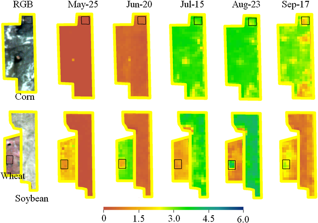 For winter wheat, the average was about 1.8 on May 25. The winter crop had grown quite well after snow melt, with the absence of N application clearly shown on the map (). The average increased to 3.2 on June 20, and decreased to 1.3 on July 15. Since the winter wheat was harvested before the acquisition of the last two images on August 23 and September 17, did not represent the condition of the winter wheat studied. The plots without N showed the strongest contrast to the rest of the field on June 20, with an average about half that of the normal value. The plot without N application also appeared to have a higher on August 23 and September 17. This probably happened because weeds had less competition from the winter wheat crop earlier in the season which enhanced their development. The corn had similar dynamics to soybeans up to August 23 as observed from the maps; however, photosynthesis was still quite active till September 17, and the maps showed that the corn crop had a slower senescent rate than that of the soybean crop, as the estimated from the OLI data was about 3.0 until September 17, indicating a significant proportion of green PAI was still present. The absence of N application was more apparent in the later growth stage, when lower were estimated on August 23 and September 17. If a single liner equation of EVI2 was generated for estimating the green of corn, soybean, and winter wheat all together, the coefficient of determination was 0.85 and the RMSE was 0.53. 4.ConclusionsThe OLI sensor onboard the newly launched Landsat-8 satellite starts to provide high quality EO data. Together with its predecessors, it will be a very important data source for local to regional studies. With an alternative design, the MSI onboard the RapidEye satellites provides high quality scientific data of high-spatial resolution and with a short revisiting cycle. The results from this study showed that, following proper radiometric calibration and atmospheric correction, vegetation indices derived from the data acquired by the two sensors were in very good agreement. This indicates that the two sensors have good and stable absolute radiometric calibration. Cross calibration of vegetation indices derived from data acquired by the two sensors using a linear transformation allowed for the combined use of the two sensors for a quantitative study as high spatial and temporal resolution remote sensing data are required for continuous monitoring of crop growth conditions throughout the whole growth cycle. The EVI2 and the MTVI2 derived from the two sensors could be cross calibrated using a simple multiplier. Comparison between the ground measured effective green PAI and the vegetation indices clearly confirmed that the EVI2 had a better sensitivity than the NDVI at high PAI, and is preferred for estimating crop PAI over the season. Good results were obtained by using only one EVI2-based linear equation for the three crops to monitor the green effective PAI. Using the EVI2 for PAI estimation of corn, soybean, and winter wheat combined with a linear equation, a coefficient of determination of 0.85 and an RMSE of 0.53 were achieved. AcknowledgmentsThis study was funded by Agriculture and Agri-Food Canada and the Canadian Space Agency through a research project on land productivity using Earth observation and crop modeling. The authors would like to acknowledge the contribution of many students from the Western University who helped with the field data collection. The authors also like to thank the local farmers who have granted access to their fields. ReferencesJ. Liuet al.,
“Estimating crop stresses, aboveground dry biomass and yield of corn using multi-temporal optical data combined with a radiation use efficiency model,”
Remote Sens. Environ., 114
(6), 1167
–1177
(2010). http://dx.doi.org/10.1016/j.rse.2010.01.004 RSEEA7 0034-4257 Google Scholar
H. Fanget al.,
“Corn‐yield estimation through assimilation of remotely sensed data into the CSM‐CERES‐Maize model,”
Int. J. Remote Sens., 29
(10), 3011
–3032
(2008). http://dx.doi.org/10.1080/01431160701408386 IJSEDK 0143-1161 Google Scholar
G. JégoE. PatteyJ. Liu,
“Using leaf area index, retrieved from optical imagery, in the STICS crop model for predicting yield and biomass of field crops,”
Field Crops Res., 131
(0), 63
–74
(2012). http://dx.doi.org/10.1016/j.fcr.2012.02.012 FCREDZ 0378-4290 Google Scholar
M. A. Wulderet al.,
“Landsat continuity: issues and opportunities for land cover monitoring,”
Remote Sens. Environ., 112
(3), 955
–969
(2008). http://dx.doi.org/10.1016/j.rse.2007.07.004 RSEEA7 0034-4257 Google Scholar
G. Chanderet al.,
“Radiometric and geometric assessment of data from the RapidEye constellation of satellites,”
Int. J. Remote Sens., 34
(16), 5905
–5925
(2013). http://dx.doi.org/10.1080/01431161.2013.798877 IJSEDK 0143-1161 Google Scholar
C. SchusterM. FörsterB. Kleinschmit,
“Testing the red edge channel for improving land-use classifications based on high-resolution multi-spectral satellite data,”
Int. J. Remote Sens., 33
(17), 5583
–5599
(2012). http://dx.doi.org/10.1080/01431161.2012.666812 IJSEDK 0143-1161 Google Scholar
E. Adamet al.,
“Land-use/cover classification in a heterogeneous coastal landscape using RapidEye imagery: evaluating the performance of random forest and support vector machines classifiers,”
Int. J. Remote Sens., 35
(10), 3440
–3458
(2014). http://dx.doi.org/10.1080/01431161.2014.903435 IJSEDK 0143-1161 Google Scholar
S. Fritschet al.,
“Validation of the collection 5 MODIS FPAR product in a heterogeneous agricultural landscape in arid Uzbekistan using multitemporal RapidEye imagery,”
Int. J. Remote Sens., 33
(21), 6818
–6837
(2012). http://dx.doi.org/10.1080/01431161.2012.692834 IJSEDK 0143-1161 Google Scholar
S. Jialiet al.,
“Estimation of crop ground cover and leaf area index (LAI) of wheat using RapidEye satellite data: prelimary study,”
in Proc. 2012 First Int. Conf. on Agro-Geoinformatics (Agro-Geoinformatics),
1
–5
(2012). Google Scholar
A. Ramoeloet al.,
“Regional estimation of savanna grass nitrogen using the red-edge band of the spaceborne RapidEye sensor,”
Int. J. Appl. Earth Obs. Geoinf., 19
(0), 151
–162
(2012). http://dx.doi.org/10.1016/j.jag.2012.05.009 1939-1404 Google Scholar
B. J. van den HurkP. ViterboS. O. Los,
“Impact of leaf area index seasonality on the annual land surface evaporation in a global circulation model,”
J. Geophys. Res. Atmos., 108
(D6), 4191
(2003). http://dx.doi.org/10.1029/2002JD002846 JGRDE3 0148-0227 Google Scholar
L. Jarlanet al.,
“Analysis of leaf area index in the ECMWF land surface model and impact on latent heat and carbon fluxes: application to West Africa,”
J. Geophys. Res. Atmos., 113
(D24), D24117
(2008). http://dx.doi.org/10.1029/2007JD009370 JGRDE3 0148-0227 Google Scholar
J. MonteithM. Unsworth, Principles of Environmental Physics: Plants, Animals, and the Atmosphere, Academic Press, Boston
(2013). Google Scholar
L. Prévotet al.,
“Assimilating optical and radar data into the STICS crop model for wheat,”
Agronomie, 23
(4), 297
–303
(2003). http://dx.doi.org/10.1051/agro:2003003 AGRNDZ 0249-5627 Google Scholar
L. Denteet al.,
“Assimilation of leaf area index derived from ASAR and MERIS data into CERES-Wheat model to map wheat yield,”
Remote Sens. Environ., 112
(4), 1395
–1407
(2008). http://dx.doi.org/10.1016/j.rse.2007.05.023 RSEEA7 0034-4257 Google Scholar
C. Bacouret al.,
“Neural network estimation of LAI, fAPAR, fCover and LAI×Cab, from top of canopy MERIS reflectance data: principles and validation,”
Remote Sens. Environ., 105
(4), 313
–325
(2006). http://dx.doi.org/10.1016/j.rse.2006.07.014 RSEEA7 0034-4257 Google Scholar
F. Baretet al.,
“LAI, fAPAR and fCover CYCLOPES global products derived from VEGETATION: Part 1: principles of the algorithm,”
Remote Sens. Environ., 110
(3), 275
–286
(2007). http://dx.doi.org/10.1016/j.rse.2007.02.018 RSEEA7 0034-4257 Google Scholar
Y. Knyazikhinet al.,
“Synergistic algorithm for estimating vegetation canopy leaf area index and fraction of absorbed photosynthetically active radiation from MODIS and MISR data,”
J. Geophys. Res. Atmos., 103
(D24), 32257
–32275
(1998). http://dx.doi.org/10.1029/98JD02462 JGRDE3 0148-0227 Google Scholar
J. LiuE. PatteyG. Jégo,
“Assessment of vegetation indices for regional crop green LAI estimation from Landsat images over multiple growing seasons,”
Remote Sens. Environ., 123
(0), 347
–358
(2012). http://dx.doi.org/10.1016/j.rse.2012.04.002 RSEEA7 0034-4257 Google Scholar
E. S. W. Group, A National Ecological Framework for Canada,
(1996). Google Scholar
F. Salvagiottiet al.,
“Growth and nitrogen fixation in high-yielding soybean: impact of nitrogen fertilization,”
Agron. J., 101
(4), 958
–970
(2009). http://dx.doi.org/10.2134/agronj2008.0173x AGJOAT 0002-1962 Google Scholar
E. F. Vermoteet al.,
“Second simulation of the satellite signal in the solar spectrum, 6S: an overview,”
IEEE Trans. Geosci. Remote Sens., 35
(3), 675
–686
(1997). http://dx.doi.org/10.1109/36.581987 IGRSD2 0196-2892 Google Scholar
V. Demarezet al.,
“Estimation of leaf area and clumping indexes of crops with hemispherical photographs,”
Agric. For. Meteorol., 148
(4), 644
–655
(2008). http://dx.doi.org/10.1016/j.agrformet.2007.11.015 0168-1923 Google Scholar
M. WeissF. Baret, Can-Eye V6. 1 User Manual, 47 INRA, Avignon, France
(2010). Google Scholar
P. M. Teilletet al.,
“Radiometric cross-calibration of the Landsat-7 ETM+ and Landsat-5 TM sensors based on tandem data sets,”
Remote Sens. Environ., 78
(1–2), 39
–54
(2001). http://dx.doi.org/10.1016/S0034-4257(01)00248-6 RSEEA7 0034-4257 Google Scholar
P. M. Teilletet al.,
“A generalized approach to the vicarious calibration of multiple Earth observation sensors using hyperspectral data,”
Remote Sens. Environ., 77
(3), 304
–327
(2001). http://dx.doi.org/10.1016/S0034-4257(01)00211-5 RSEEA7 0034-4257 Google Scholar
P. M. Teilletet al.,
“Impacts of spectral band difference effects on radiometric cross-calibration between satellite sensors in the solar-reflective spectral domain,”
Remote Sens. Environ., 110
(3), 393
–409
(2007). http://dx.doi.org/10.1016/j.rse.2007.03.003 RSEEA7 0034-4257 Google Scholar
J. Rouse Jr.,
“Monitoring the vernal advancement and retrogradation (green wave effect) of natural vegetation,”
in NASA/GSFC, Final Report,
1
–137
(1974). Google Scholar
A. A. GitelsonY. J. KaufmanM. N. Merzlyak,
“Use of a green channel in remote sensing of global vegetation from EOS-MODIS,”
Remote Sens. Environ., 58
(3), 289
–298
(1996). http://dx.doi.org/10.1016/S0034-4257(96)00072-7 RSEEA7 0034-4257 Google Scholar
J.-L. RoujeanF.-M. Breon,
“Estimating PAR absorbed by vegetation from bidirectional reflectance measurements,”
Remote Sens. Environ., 51
(3), 375
–384
(1995). http://dx.doi.org/10.1016/0034-4257(94)00114-3 RSEEA7 0034-4257 Google Scholar
A. R. Huete,
“A soil-adjusted vegetation index (SAVI),”
Remote Sens. Environ., 25
(3), 295
–309
(1988). http://dx.doi.org/10.1016/0034-4257(88)90106-X RSEEA7 0034-4257 Google Scholar
G. RondeauxM. StevenF. Baret,
“Optimization of soil-adjusted vegetation indices,”
Remote Sens. Environ., 55
(2), 95
–107
(1996). http://dx.doi.org/10.1016/0034-4257(95)00186-7 RSEEA7 0034-4257 Google Scholar
D. Haboudaneet al.,
“Hyperspectral vegetation indices and novel algorithms for predicting green LAI of crop canopies: modeling and validation in the context of precision agriculture,”
Remote Sens. Environ., 90
(3), 337
–352
(2004). http://dx.doi.org/10.1016/j.rse.2003.12.013 RSEEA7 0034-4257 Google Scholar
Z. Jianget al.,
“Development of a two-band enhanced vegetation index without a blue band,”
Remote Sens. Environ., 112
(10), 3833
–3845
(2008). http://dx.doi.org/10.1016/j.rse.2008.06.006 RSEEA7 0034-4257 Google Scholar
BiographyJiali Shang received her BSc in physical geography from Beijing Normal University, Beijing, China, in 1984, the MA degree in geography from the University of Windsor, Windsor, Canada, in 1996, and a PhD degree in environmental studies from the University of Waterloo, Waterloo, Canada, in 2005. She is a research scientist with the Agriculture and Agri-Food Canada (AAFC), Ottawa, ON, Canada. She specializes in the application of optical and radar integration for agriculture. Ted Huffman specializes in spatial analysis of agricultural land use, land management and farming systems. He has undergraduate degrees in agriculture and geography and a PhD in remote sensing. His work is applied in national multidisciplinary projects related to the health of soil, air, and water. He has served on the Environmental Indicators program of the OECD, the Good Practice Guidance of the IPCC and Canada’s National Inventory Reports to the UNFCCC. Jinfei Wang received BS and MSc from Peking University, Beijing, China, and a PhD from University of Waterloo, Waterloo, Canada. She is currently a professor with the Department of Geography, the University of Western Ontario, Canada. Her research interests include methods for information extraction from remotely sensed imagery and its applications in urban, wetland and agricultural cropland environments using high resolution multispectral, hyperspectral, lidar, and radar data. David Kroetsch is a senior soil resource specialist with Agriculture and Agri-Food Canada, specializing in soil survey upgrades and research on soil re-survey and the spatial and temporal change in soil and landscape attribute information using geospatial digital information and modeling. He is an adjunct professor in the School of Environmental Sciences, University of Guelph, involved with the development and instruction of a Graduate Diploma field course in soil and landscape inventory. Nicholas Lantz received his BSc in biology and GIS, and MSc degree in remote sensing, both from the University of Western Ontario (UWO), Canada. He has worked at the Canada Centre for Remote Sensing and Agriculture and Agri-Food Canada. His main research interests include utilizing high-resolution satellite imagery for invasive plant monitoring, land cover change detection, and seasonal snow mapping. |


