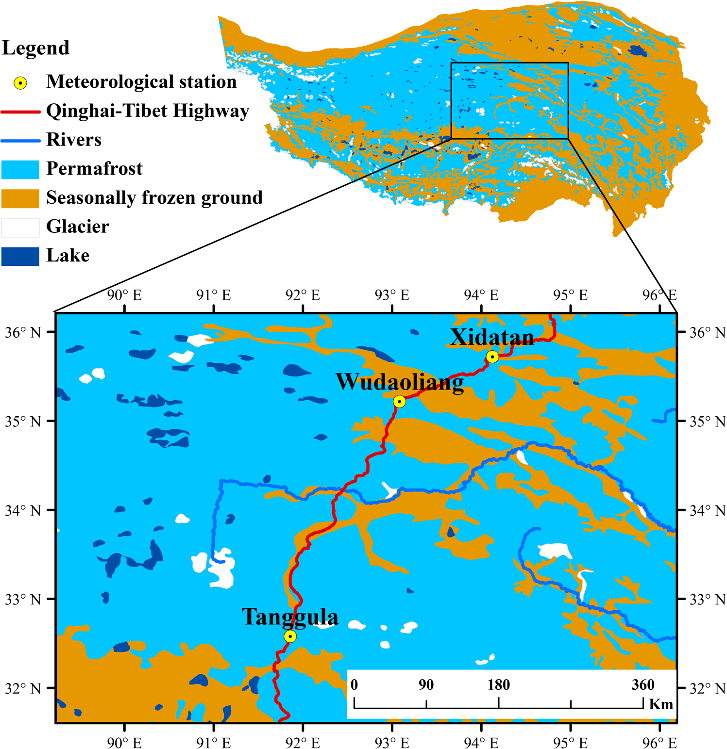
1.

Introduction

Ground surface temperature (GST) is an integrated result of heat and moisture exchanges through the ground surface.¹ In permafrost regions, GST can serve as upper boundary conditions in permafrost models for modeling the freeze-thaw depths of the active layer and the thermal properties of permafrost, and is, therefore, a crucial parameter for the thermal state of the active layer and permafrost.¹ Thus, accurate estimation of GST in permafrost regions spatially and temporally could provide valuable dataset in the research on not only permafrost, but also hydrology, ecology, and climate.^2–4 Unfortunately, GST is not a standard meteorological measurement and is rarely available for a specific case.

Accompanied with the development of remote sensing technology, satellite data make it possible to measure land surface temperature (LST) over the entire globe with sufficiently high temporal resolution and with complete spatial coverage rather than only point values.⁵ Currently, LST can be derived from sensors, including the Landsat Thematic Mapper/Enhanced Thematic Mapper Plus, the advanced spaceborne thermal emission and reflection radiometer, the advanced very high-resolution radiometer, the advanced along-track scanning radiometer, the spinning enhanced visible and infrared imager, and the moderate-resolution imaging spectroradiometer (MODIS),^6–12 and especially with improved moderate-resolution satellite sensors, such as the MODIS instruments onboard the Terra and Aqua platforms.

The MODIS Terra and Aqua satellites are in Sun-synchronous orbit near polar orbits, with Aqua in an ascending orbit and Terra in a descending orbit and equatorial crossings at 10:30 a.m. for Terra and at 1:30 p.m. for Aqua (local solar time). MODIS Terra data became available in February 2000, and Aqua data became available in July 2002. The generalized split-window algorithm is used to derive LST from bands 31, 32 and known emissivities.¹³ Comparisons between the MODIS LST products and in situ measurements indicate that the accuracy of the MODIS LST products is better than 1 K for a given observation time and angle. Therefore, the MODIS LST products have been widely used in various studies,^14,15 including research on the cryosphere,¹⁶ which is sensitive to climate changes.

Integrated mean daily values from Aqua and Terra daytime and nighttime LST acquisitions in Quebec and the northern slope of Alaska were performed by Hachem et al.^16,17 The results showed good agreement with air temperature and were used to study the spatial distribution of permafrost. However, some research found that the performance of MODIS LST over the regions of wet polygonal tundra in Siberia¹ and high Arctic tundra in Svalbard¹⁸ was affected by cloud cover, water bodies, snow cover, and soil properties.

Despite the fact that MODIS LST has been widely used in the circum-Arctic regions, there are few reports to evaluate the LST in permafrost regions of high-altitude areas. Permafrost on the Tibetan Plateau (TP) occupies $\sim 1.5\times {10}^6{\mathrm{km}}^2$ in area^19–21 and exerts great influences on regional and global climates through thermal forcing mechanisms.²² Many studies have analyzed climate change in the TP using observational data from meteorological stations,²³ and the permafrost is considered as one of the most sensitive indicators. For low-statured vegetation, GST is likely a better indicator than air temperature when used to evaluate the thermal condition of permafrost regions.²⁴ Wu et al.²⁵ analyzed the changes of the mean annual GST and the surface freezing and thawing indices over the period of 1980 to 2007 based on the GST records from 16 meteorological stations, and the results indicated that the dramatic ground surface warming could have significant influence on the change of the permafrost thermal regime in the study region. However, meteorological stations are sparse in the west of TP, and a spatial expansion of temperature combined with remote sensing data is essential to assess the regional ground thermal regime in cold regions.

The MODIS sensors observed the instantaneous LST during the satellite overpass times, while the data that we need to analyze or drive the permafrost model mostly are the mean daily GST. Previous studies focused on the method to derive spatial distribution of mean daily air temperature in the TP, and most of these studies aimed at using MODIS LST combined with the statistical approach or the temperature-vegetation index.^26,27 There are only few studies on deriving the mean daily GST from MODIS LST, which is mainly due to the scarcity of meteorological stations and lack of consecutive and high temporal resolution instrumental records.

It is well known that single daytime MODIS observations, which are significantly influenced by solar radiation and cloud cover, are used for the model. The higher observation frequency (for example, combined daytime and nighttime LST) used in models would generate more accurate spatial GST products.²⁸ Meanwhile, the accuracy is influenced by the number and period of the available pixels of MODIS LST.

This study estimates mean daily GST using empirical models combining single daily tiled daytime and nighttime MODIS LST observations (considering the acquisition time during the day). A key difference from the previous approaches is that the model training datasets consisted of the automatic weather station (AWS) observations at the satellite overpass times. Three models were employed in this study according to different compositions of daytime/nighttime MODIS LST as predictors. Data from 2012 at three AWS were used to establish the empirical models, and the models were assessed with cross-validation.

2.

Study Area

In order to establish the suitable methods to estimate the GST in permafrost regions of TP, the study area was arbitrarily selected within the permafrost region of TP. It is located in central TP with an area of $\sim 0.32\times {10}^6{\mathrm{km}}^6$. Three AWS were set up in the study area along the Qinghai-Tibet Highway (Fig. 1 and Table 1). These stations provide diurnal temperature curves, which are used in conjunction with MODIS LST to predict mean daily GST.

Fig. 1

Location of the study area (yellow dots represent automatic weather stations).

Table 1

Description and location of automatic weather stations in the central Tibetan Plateau.

3.

Data and Methods

3.3.

Data Processing and Model Establishment

Due to the intrinsic scanning characteristics of the MODIS instrument onboard the polar-orbiting satellites, the differences in local solar VT for the same pixel on different days in one revisit period (16 days for reaching the same ground track) may reach up to 2 h. Figure 2 shows MODIS Terra satellite daytime overpass times at the TGL station within one revisit period (from January 1 to January 16, 2012), and the other three overpass times (Terra satellite nighttime, Aqua satellite daytime, and Aqua satellite nighttime overpass) have corresponding and similar fluctuations. To match the AWS observation time, the local solar VT was converted to local standard time (Beijing time).

Fig. 2

Local standard time for the same pixel in one revisit period of daytime MODIS Terra satellite at Tanggula station.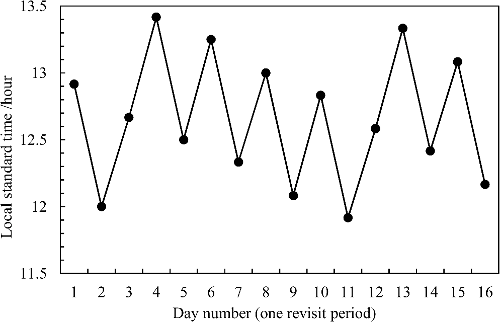

The models establishing procedure was composed of three steps, outlined in detail below.

• Step 1: Select the AWS half-hour GST observations closest to satellite overpass times (hereafter MODIS-GST) as predictor(s) for each of the three AWS. Then, we explore the linear correlations between the mean daily GST (hereafter meteo-GST) and different predictor(s) combinations of daytime/nighttime MODIS-GST with data for all 366 days of the year 2012. The meteo-GST were averages of the 48 half-hour observation values in one day. The candidate predictor combinations include ${\mathrm{GST}}_{\text{moddt}}$, ${\mathrm{GST}}_{\text{moddt}}$, ${\mathrm{GST}}_{\text{myddt}}$, and ${\mathrm{GST}}_{\text{myddt}}$; ${\mathrm{GST}}_{\text{moddt}}$ and ${\mathrm{GST}}_{\text{moddt}}$; ${\mathrm{GST}}_{\text{myddt}}$ and ${\mathrm{GST}}_{\text{myddt}}$; and ${\mathrm{GST}}_{\text{moddt}}$, ${\mathrm{GST}}_{\text{moddt}}$, ${\mathrm{GST}}_{\text{myddt}}$, and ${\mathrm{GST}}_{\text{myddt}}$, as shown in Table 3.

• Step 2: By comparing determination coefficients ($R^2$) and root mean square errors (RMSE) of the linear regressions, proper predictor(s) and statistic correlations were selected as empirical models. Then, the models established by observations from one of the three AWS were applied to MODIS LST data to estimate meteo-GST, and observations from the remaining two were used to validate the models.

• Step 3: The models’ validation was performed by using statistical parameters, such as the mean error (ME), mean absolute error (MAE), and RMSE. The ME, MAE, and RMSE were calculated as follows:

  $$\mathrm{ME}=\sum _{i=1}^n(y_{\text{predict}}-y_{\text{measured}})/n,$$
  $$\mathrm{MAE}=\sum _{i=1}^n(|y_{\text{predict}}-y_{\text{measured}}|)/n,$$
  $$\mathrm{RMSE}=\sqrt{\frac{1}{n}\sum _{i=1}^n{(y_{\text{predict}}-y_{\text{measured}})}^2,}$$
  where $n$ is the number of observations, $i$ is the observation number, and $y$ is the mean daily GST in this study.

Table 3

Description of the terminology.

Terms	Description
${\mathrm{GST}}_{\text{moddt}}$ (°C)	GST observed by AWS at Terra daytime overpass time
${\mathrm{GST}}_{\text{modnt}}$ (°C)	GST observed by AWS at Terra nighttime overpass time
${\mathrm{GST}}_{\text{myddt}}$ (°C)	GST observed by AWS at Aqua daytime overpass time
${\mathrm{GST}}_{\text{mydnt}}$ (°C)	GST observed by AWS at Aqua nighttime overpass time
${\mathrm{GST}}_{\text{mean}}$ (°C)	Mean daily GST observed by AWS
${\mathrm{LST}}_{\text{moddt}}$ (°C)	Daytime LST obtained by Terra
${\mathrm{LST}}_{\text{modnt}}$ (°C)	Nighttime LST obtained by Terra
${\mathrm{LST}}_{\text{myddt}}$ (°C)	Daytime LST obtained by Aqua
${\mathrm{LST}}_{\text{mydnt}}$ (°C)	Nighttime LST obtained by Aqua
${\mathrm{LST}}_{\text{mean}}$ (°C)	Mean daily LST estimated by the models

Note: GST, ground surface temperature; AWS, automatic weather station; LST, land surface temperature; moddt, Terra daytime; modnt, Terra nighttime; myddt, Aqua daytime; mydnt, Aqua nighttime.

4.

Results

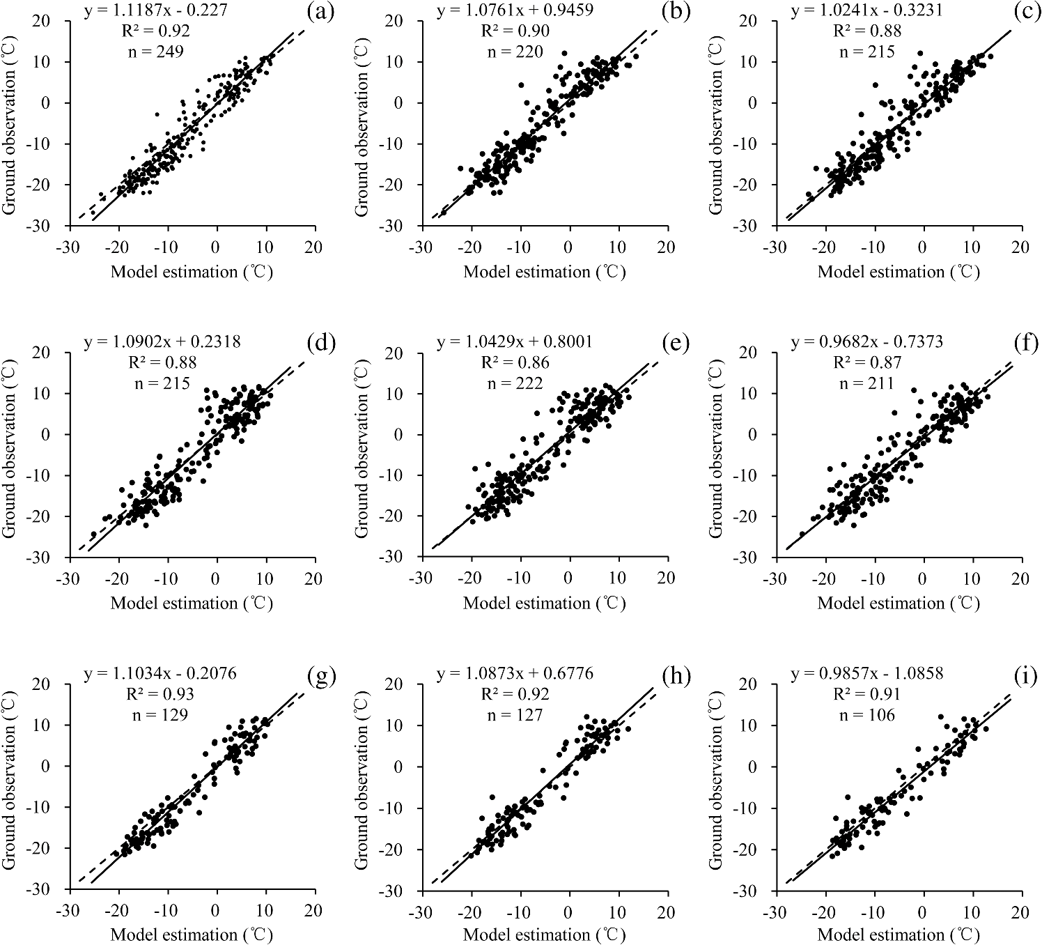
4.2.

Results of Model Validation

Estimations of mean daily LST (${\mathrm{LST}}_{\text{mean}}$) were made by the three models with the MODIS LST data (Table 5). Figure 3 demonstrates the models’ estimated ${\mathrm{LST}}_{\text{mean}}$ against the ground observations of ${\mathrm{GST}}_{\text{mean}}$; the slopes of the regression lines of the scatter plots were 0.97 to 1.12 at three AWS. Compared to models I and II, model III yielded a higher $R^2$ (0.93, 0.92, and 0.91 for XDT, WDL, and TGL, respectively) (Fig. 3).

Fig. 3

Model estimations against ground observations of ground surface temperature.

Table 6 lists the statistics of the estimation residuals. The XDT observations in Table 6 indicate the empirical models established by the observations at XDT station and validated with observations at WDL and TGL stations (so to with the WDL and TGL observations). The annual averages of the ME of the three models were near zero and ranged from $-1$ to 1, with slightly negative values with WDL observations and positive values with XDT and TGL observations. Table 6 showed that model III yielded the lowest MAE and RMSE, 2.28 to 2.42°C and 2.96 to 3.05°C, of all the three AWS observations, respectively. The WDL observations performed best in model III, with ME, MAE, and RMSE of $-0.21$, 2.28, and 2.97°C, respectively. For model III, there was no obvious difference in the MAE and RMSE of the three AWS observations, which were $\sim 2.4$ and 3°C, respectively. Although the GST estimated from model III at each of the three AWS provided the best agreement with meteo-GST, the number of MODIS LST available was reduced to $\sim 14.2$ to 20.5%, which indicates that model III was not always feasible for the study area. This is a reminder that model I and model II should be supplemental methods. Compared to model II, model I had a lower MAE (2.48 to 2.71°C) and RMSE (3.24 to 3.53°C), which indicates that the Terra MODIS LST performed better than the Aqua MODIS LST when estimating meteo-GST in the study area. Generally, those models performed well in spite of some possible bias caused by the clouds.

Table 6

Statistics of the estimation residuals of the three models.

Model no.	XDT observations			WDL observations			TGL observations
	ME	MAE	RMSE	ME	MAE	RMSE	ME	MAE	RMSE
Model I	0.95	2.66	3.24	$-0.48$	2.48	3.36	0.47	2.71	3.53
Model II	0.14	3.06	3.86	$-0.61$	2.89	3.81	0.6	2.92	3.72
Model III	0.75	2.39	2.96	$-0.21$	2.28	2.97	1	2.42	3.05

Note: XDT observations, the empirical model established by the observation data at XDT station and validated with WDL and TGL stations; WDL observations, the empirical model established by the observation data at WDL station and validated with XDT and TGL stations; TGL observations, the empirical model established by the observation data at TGL station and validated with XDT and WDL stations; ME, mean error; MAE, mean absolute error; RMSE, root mean squared error.

5.

Discussion

The mean daily GST (meteo-GST) estimated by the empirical models combining MODIS LST showed a good agreement with AWS observations. There are two major reasons leading to this. First is the similar observation principle between infrared radiometer and sensors on board satellites though MODIS sensors considered the atmospheric transmission. Second, the training datasets we used in following statistical analysis and models establishment with mean daily GST are the AWS observations at the satellite overpass times rather than the MODIS LST.

To compare the accuracy with routine modeling methods that have been used in previous study,¹⁷ MODIS LST data have also been applied as training datasets to establish the empirical models. Table 7 shows the resulting estimation residuals. Almost all the ME, MAE, and RMSE of the three models in Table 7 were larger than those in Table 6, which indicates that the models established by the AWS observations at the satellite overpass times were better than the models established by MODIS LST. The MAE and RMSE for model III improved $\sim 0.22$ to 0.85°C and 0.36 to 0.83°C, respectively. Though the models established by the AWS observations at the satellite overpass times cannot solve the mismatch of point and 1 km per pixel scales, the increased number of training data theoretically still improves the accuracy of estimated meteo-GST.

Table 7

Statistics of the estimation residuals of the three models by training data of MODIS LST.

During the daytime, the difference between MODIS LST and AWS observations is mainly controlled by the surface energy balance, which is a complex system dependent on information not easily available (such as solar radiation, cloud cover, wind speed, soil moisture, and surface roughness).³⁰ During the night, solar radiation does not affect the thermal infrared signal. Therefore, nighttime LST is a better predictor than daytime LST for estimating meteo-GST. This also can be proved from the regression coefficient in Table 5. Models coupling nighttime and daytime LST were more accurate than those using nighttime or daytime LST alone.²⁸ Correlation analysis between the mean daily GST and the MODIS-GST showed that the Terra MODIS performed better than the Aqua MODIS, while Aqua MODIS outperformed Terra MODIS when applied the models to estimated meteo-GST. The model results using nighttime and daytime LST reflect real LST because they reduce the possible bias caused by the clouds. Further analysis demonstrates that the coupled nighttime and daytime LST of Terra and Aqua will perform better than using Terra or Aqua alone. For regions with extensive cloud cover that cannot obtain the daytime and nighttime LST at the same day, Williamson et al.²⁴ proposed the interpolated curve mean daily surface temperature method, which requires only a single daytime observation.

There is no significant difference in the MAE and RMSE of the three AWS observations, $\sim 2.4$ and 3°C, respectively, which indicates that the deviation error is no different when a specific the AWS observation is selected to establish the models. However, whether the ME would be negative or positive depends on the difference of meteo-GST between the modeling station and validation stations being lower or higher. The morphology of areas where the three AWS located are flat and the underlying surfaces are alpine meadow and alpine desert, which can represent the general characteristic of the central TP. Using an averaged result or dividing the area into several subregions (such as utilizing the Thiessen polygon)³¹ when used for regional GST estimates will be a better method.

The difference between estimated and observed mean daily GST was likely due to the combination of several factors, including temperature differences due to time offset between AWS half-hour observation and satellite overpass time and cloud contamination and cloud shadow causing differences in LST across spatial and temporal scales. Although the MODIS cloud-detecting algorithm takes as many as 22 of the 36 MODIS bands to maximize the reliability of cloud detection, uncertainties still exist in the MODIS cloud mask product applications.⁷ For some instances, the residual clouds contaminate the data, and in others, the overdetection of clouds diminishes the availability of clear observations, which leads to many fill-values in the downstream products (such as LST); these effects could affect data availability. For example, the false-positive cloud flags in hot and bright pixels likely lead to a summertime cooling bias in LST over urban areas and the presence of residual clouds would cause misidentification of vegetation changes.^32–34 Future work should be devoted to the identification of cloud-contaminated LST data and the degree to which contaminated LST values are affected. By quantifying the degree of contamination, data volume will be preserved and quality improved. Furthermore, mismatches in spatial and temporal scale should also be investigated. Statistical techniques should be improved to make the most use of limited ground station data. The implementation of empirical models in this study could provide a powerful technique to obtain the spatial distribution of GST using the MODIS LST products.

6.

Conclusion

To assess the potential of remotely sensed data to estimate GSTs, an empirical model was established based on three AWS in the central TP. The empirical models were established by the correlation between the mean daily ground surface temperature (meteo-GST) of the three AWS observations and the AWS observations at the satellite overpass times, with three different combinations of daytime/nighttime MODIS LST (Terra daytime and nighttime, Aqua daytime and nighttime, and Terra and Aqua daytime and nighttime). Employing both daytime and nighttime from Terra or Aqua MODIS as predictors performed better than using daytime or nighttime alone. Among the three models, the model established by observations of Terra and Aqua daytime and nighttime, MODIS LST, yielded the highest $R^2$ and the lowest MAE and RMSE, but the number of available pixels was substantially reduced. There was no obvious difference in $R^2$, MAE, and RMSE of three AWS observations, $\sim 0.92$, 2.4°C, and 3°C, respectively. Terra MODIS LST performed better than Aqua MODIS LST to estimate meteo-GST. Models established by the AWS observation values at the MODIS overpass times were better than the models established by the MODIS LST observations. These three AWS are located in the central TP and, therefore, indicate the thermal conditions of permafrost, so the estimation of mean daily GST could be a powerful dataset for the monitoring and modeling of permafrost.