Land cover classification in multispectral imagery using clustering of sparse approximations over learned feature dictionaries

Daniela I. Moody; Steven P. Brumby; Joel C. Rowland; Garrett L. Altmann

doi:10.1117/1.JRS.8.084793

9 December 2014 Land cover classification in multispectral imagery using clustering of sparse approximations over learned feature dictionaries

Daniela I. Moody, Steven P. Brumby, Joel C. Rowland, Garrett L. Altmann

Author Affiliations +

Journal of Applied Remote Sensing, Vol. 8, Issue 1, 084793 (December 2014). https://doi.org/10.1117/1.JRS.8.084793

Abstract

We present results from an ongoing effort to extend neuromimetic machine vision algorithms to multispectral data using adaptive signal processing combined with compressive sensing and machine learning techniques. Our goal is to develop a robust classification methodology that will allow for automated discretization of the landscape into distinct units based on attributes such as vegetation, surface hydrological properties, and topographic/geomorphic characteristics. We use a Hebbian learning rule to build spectral-textural dictionaries that are tailored for classification. We learn our dictionaries from millions of overlapping multispectral image patches and then use a pursuit search to generate classification features. Land cover labels are automatically generated using unsupervised clustering of sparse approximations (CoSA). We demonstrate our method on multispectral WorldView-2 data from a coastal plain ecosystem in Barrow, Alaska. We explore learning from both raw multispectral imagery and normalized band difference indices. We explore a quantitative metric to evaluate the spectral properties of the clusters in order to potentially aid in assigning land cover categories to the cluster labels. Our results suggest CoSA is a promising approach to unsupervised land cover classification in high-resolution satellite imagery.

1. Introduction

Techniques for automated feature extraction, including machine vision and pattern recognition algorithms, have been of much interest in the areas of change detection and land cover classification in remote sensing datasets of satellite and aerial imagery.¹ Despite vast archives of globally distributed remotely sensed data collected over the last four decades and the availability of computing resources to process these datasets, global assessment of all but the simplest landscape features is presently not feasible. This limitation arises from the substantial human intervention needed to accurately train current state-of-the-art feature extraction software and the limited applicability of resulting feature extraction solutions to multiple images. Without more robust and adaptive methods to identify and extract land surface features, Earth scientists lack critical datasets needed to parameterize models and quantify climatic and land use driven changes. Given the much improved resolution of Woldview-2 multispectral satellite data at $1.8 m / pixel$ nadir compared to, e.g., multispectral Landsat data at $30 m / pixel$ , such surface changes are now more readily visible and can be more closely monitored.

Recent work in the area of climate change modeling and monitoring has indicated that air temperatures have been rising in both Alaska²^,³ and the western Canadian Arctic²^,⁴^,⁵ over the last few decades. Global climate models suggest that the Arctic will continue to warm more rapidly than southerly locations,² drawing significant attention to this region among climatologists. The Arctic biome is responding to this warming, and the effects are multiple and interconnected. In the terrestrial biome, the thawing of the permafrost can be indirectly studied using surface changes in vegetative cover⁶^–⁹ or in geomorphic features, such as polygonal ground and river banks.¹⁰ Specifically, warming alters transitional regions between upright and dwarf shrub tundra,¹¹ and there has been evidence of increasing shrub cover in air photos¹² and of changes to vegetation indices derived from satellites.⁶^–⁹ Colonizing shrubs affect snowpack depth, although it is yet unclear at what magnitude and in what direction.⁵ Recent studies have attributed dramatic increases in the rates of shoreline erosion along Arctic coastlines and riverbanks to global climate change and near-surface permafrost degradation.¹³^,¹⁴ Across much of the Arctic, the number of lakes and their sizes have also been changing as a result of permafrost degradation,¹⁵ altering surface water dynamics and causing possible release of soil organic carbon.¹⁶ Given the much improved resolution of Woldview-2 satellite data, such surface changes are now more readily visible and can be more closely monitored.

Land cover classification in satellite imagery presents a signal processing challenge, usually due to the lack of verified pixel-level ground truth information. A large number of proprietary and open source applications exist to process remote sensing data and generate land cover classification using, for example, normalized difference vegetative index (NDVI) information,¹⁷ or unsupervised clustering of raw pixels. These techniques rely heavily on domain expertise and usually require human input. Other land cover classification approaches involve the use of state-of-the-art genetic algorithms, such as GENIE,¹⁸^–²¹ to extract a particular class of interest in a supervised manner. GENIE and GeniePro are feature extraction tools developed at Los Alamos National Laboratory for multispectral, hyperspectral, panchromatic, and multi-instrument fused imagery, but they require supervision in training, too. One of the main limitations is the difficulty in providing clean training data, i.e., only pixels that truly belong to the class of interest. This is easier to do when the classes are well separated spatially from other classes, such as water bodies from land or golf courses from buildings,²² but much more difficult to do when the classes are spatially mixed (e.g., tundra shrubs and grasses).

Such techniques have been successful for lower-resolution satellite data, but they rely heavily on domain expertise and frequently require human input or supervision.²¹ They perform well on certain types of problems, such as distinguishing between water and land features (e.g., automatic lake detection), or specific vegetative analysis, but are usually not robust for spatially mixed classes. The quality of spectral unmixing plays an important role in extracting information and features from low-resolution pixels, and historically, it has been a typical step in processing and classifying multispectral and hyperspectral data. In the case of Worldview-2 multispectral imagery, however, spectral unmixing is less of a problem due to the much enhanced pixel resolution. The challenge instead lies in context-based information extraction using spatial and spectral texture generated by adjacent pixels. The textural patterns in a given image also need to be learned based on the wider-area context provided by the full image scene, usually necessitating significant computational resources and creative software optimization. Many current users of multispectral Worldview-2 data resort to downsampling the image to equivalent Landsat resolution in order to facilitate feature extraction using available commercial applications.

A fundamental problem to creating scalable feature extraction technology capable of processing imagery datasets at global scales is the overconstrained training needed to generate effective solutions. Many features of environmental importance, such as, but not limited to, rivers, water bodies, coastlines, glaciers, and vegetation boundaries, are readily recognizable to humans based on a simple set of attributes. The very best of current feature extraction software, e.g., LANL-developed GeniePro, however, require extensive, image-specific training that leads to a solution with limited applicability to images other than the image used for training. Developing automatic, unsupervised feature extraction and high-resolution, pixel-level classification tools can, therefore, have a significant impact in studying climate change effects and would provide the climate change community with more exact ways of detecting these changes.

We present a technical solution for unsupervised classification of land cover in multispectral satellite imagery, using sparse representations in learned dictionaries: clustering on sparse approximations (CoSA). The CoSA algorithm is derived from previous work and was first introduced and demonstrated on a selected dataset in Refs. 23 and 24. A Hebbian learning rule is used to build multispectral, multiresolution dictionaries that are adapted to regional satellite image data. Sparse image representations of pixel patches over the learned dictionaries are used to perform unsupervised $k$ -means clustering into land-cover categories. This approach combines spectral and spatial textural characteristics to detect geologic, vegetative, and hydrologic features. Here we focus on a particular Arctic ecosystem study area and explore two feature extraction processes using Hebbian learning. The first is based on learning from eight-band multispectral pixel patches, and the second is a novel approach based on learning features from normalized band difference indexes. We also introduce a possible clustering separability metric based on intrinsic data properties. A few of these findings were presented in Ref. 25, and in this manuscript, we detail the algorithm to learn from both raw multispectral imagery, as well as normalized band difference indices and provide additional detail on implementation. We include complete results on Barrow data for all the different feature extraction scenarios we explored, as well as a detailed quantitative analysis on performance and on comparison of dictionary types. Our results suggest that CoSA is a promising approach to unsupervised land cover classification in high-resolution satellite imagery.

The layout of the paper is as follows. In Sec. 2, we describe the study area and the satellite data used in this work and highlight classification results obtained with a standard remote sensing software package. In Sec. 3, we outline our Hebbian method of learning dictionaries of features and explore their spatial and spectral properties. We summarize our CoSA method, discuss land cover clustering results using two types of learned features, and introduce a label separability metric in Sec. 4, and conclude with brief remarks in Sec. 5.

2. Arctic Study Site

Located within the Alaskan Arctic Coastal Plain, on the Chukchi Sea coast, the village of Barrow is the northernmost community in the United States (Fig. 1), located around 71.2956° N, 156.7664° W. The nearby area includes the study site for a Department of Energy Next Generation Ecosystem Experiments (NGEE-Arctic) project. The long-term goal is developing an ecosystem model that integrates various observables, including vegetative changes, land-surface characteristics, surface water dynamics, and subsurface processes causing possible release of soil organic carbon, among others.

Fig. 1

WorldView-2 image of Barrow study area, northern Alaska, shown in (8,6,4) band combination (left). This region is dominated by water and polygonal ground, both high centered and low centered, that is, low moisture and high moisture soils. White rectangular markup in the left image shows the region of analysis.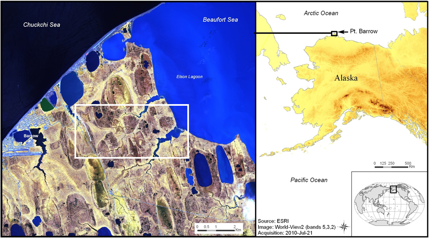

In this paper, we focus on extracting land surface features using DigitalGlobe’s WorldView-2 satellite imagery. The sensor provides the highest resolution commercially available multispectral data at $1.8 m / pixel$ spatial resolution and has eight multispectral bands: four standard bands (red, green, blue, and near-infrared 1) and four new bands. Ordered from shorter to longer wavelength, the list of bands is coastal blue, blue, green, yellow, red, red edge, near-infrared 1 (NIR1), and near-infrared 2 (NIR2).²⁶ This high spatial resolution leads to imagery characterized by very rich textures and a great level of detail, enabling more in-depth land cover analysis. The orthorectified image in Fig. 1 was acquired during the summer in mid-July and shows the greater Barrow area, with spatial extent $\sim 12.2 km \times 14.4 km$ (530 Mpixels multispectral). Here we show an (8,6,4) band combination (i.e., NIR2, red edge, and yellow), which is especially useful in vegetation analysis and biomass studies. For ease of visualization, we focus on the region delineated by the white rectangle in Fig. 1, of approximate spatial extent $1.9 km \times 5.4 km$ , and show that zoomed-in section in Fig. 2.

Fig. 2

Barrow zoom area, northern Alaska, shown in red, green, blue (RGB) band combination. This reduced area image will be subsequently used in this paper both for dictionary learning and for cluster training.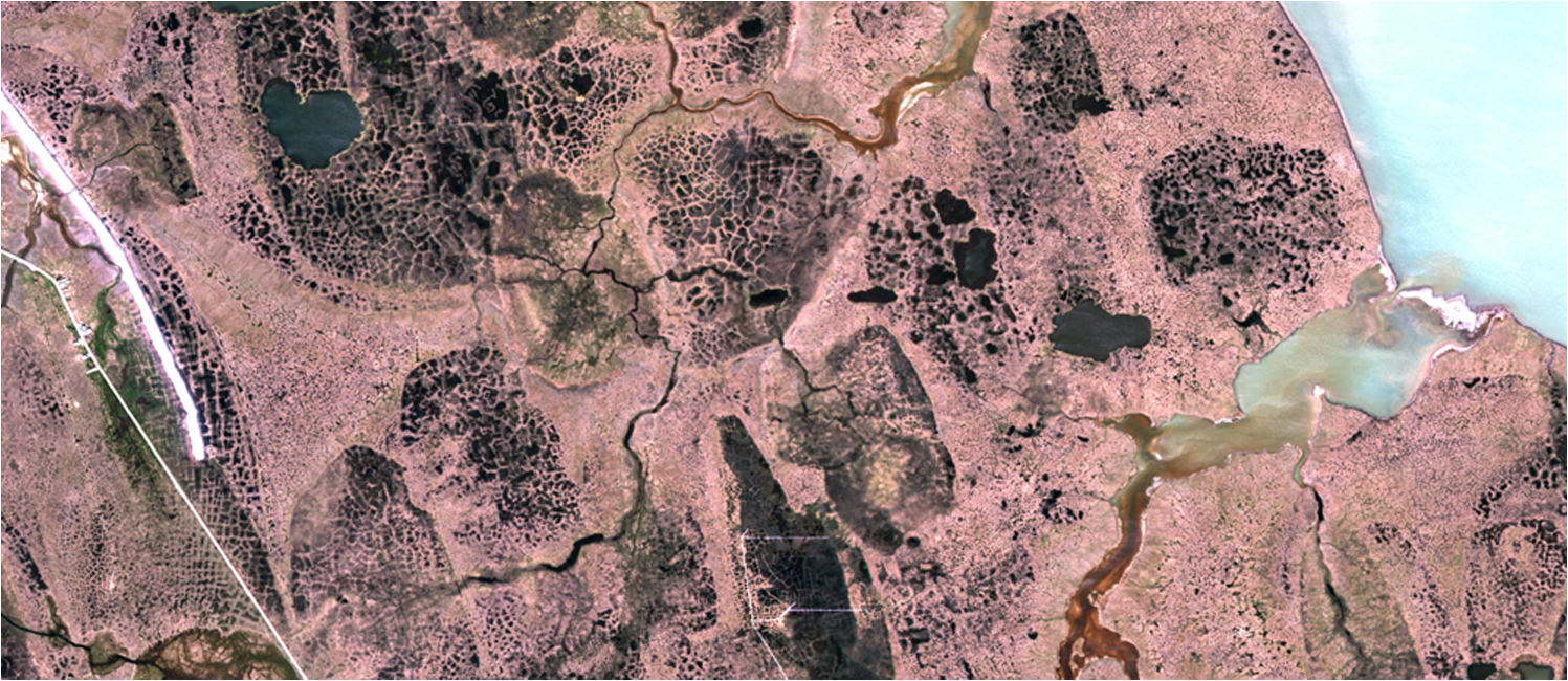

Here we use the red, green, and blue (RGB) band combination, which highlights the degree of water turbidity, due largely to suspended sediment, in the lakes and rivers, as well as the rich geomorphic texture present in the Barrow area. The region includes a mosaic of thaw lakes, drained thaw lake basins, and interstitial polygons,²⁷^,²⁸ both high centered and low centered (i.e., low moisture and high moisture soils). Polygonal ground is a geomorphic feature common in permafrost regions and is the object of much study in the Barrow region. Such frozen soil can be dry, or it can contain ice, which is usually found in large wedges forming a honeycomb of ice walls beneath the soil surface. Polygonal tundra landscapes are highly heterogeneous, varying substantially over spatial scales of only a few meters and, thus, presenting a significant challenge for developing the vegetation maps needed to scale plot-level measurements to wide-area coverage maps landscape. Vegetative gradients exist both within a single polygon type and between polygon types with differing degrees of ice-wedge degradation.²⁹ Plant communities are linked to polygon-induced microtopography and include sedges, mixed tall graminoid-forb-moss communities, graminoid-lichen communities, and low-stature, lichen dominated communities. Leaf area index for the region²⁹ is higher in trough communities (averaging between 0.7 and $1.1 m^{2} / m^{2}$ ) and decreases from wetter to drier areas along the moisture gradient (averaging between 0.1 and $0.5 m^{2} / m^{2}$ ).

This reduced area image will be subsequently used in this paper both for dictionary learning and for cluster training.

2.1.

Current Classification Methods and Performance

Several existing remote sensing unsupervised classification approaches were used to generate land cover classification maps for comparison to our CoSA method. We show two representative results from one of the most widely used remote-sensing software packages, the Environment for Visualizing Imagery (ENVI), distributed by Exelis Visual Information Solutions out of Boulder, Colorado. We applied ENVI’s unsupervised classifiers (IsoData and $K$ -means) to the eight-band multispectral Barrow image to highlight the limitations of such approaches, as previously discussed in Ref. 23. Figure 3 shows the IsoData classification result using all eight spectral bands (17 final clusters), and Fig. 4 similarly shows the result of ENVI $K$ -means clustering into 20 clusters using all eight bands. Upon visual inspection, IsoData appears better than $K$ -means at retaining the polygonal ground features, and it appears to be particularly sensitive to hydrologic features. The $K$ -means result does not appear to lead to overall meaningful clustering that is particularly good at identifying all the features and the structures present in Fig. 1.

Fig. 3

IsoData Environment for Visualizing Imagery (ENVI) classification results on the Barrow training area using 17 final clusters.

Fig. 4

K-means (ENVI) classification results on the Barrow training area using 20 clusters.

2.2.

Normalized Band Difference Analysis

In the absence of pixel-level ground truth for our satellite imagery, much of the initial performance assessment of the CoSA algorithm is qualitative and helps guide the research efforts toward parameters leading to meaningful clustering. One such qualitative technique is based on normalized band difference analysis. This is a relatively common approach to estimating land cover labels and involves manipulating spectral bands into index images, e.g., NDVI,¹⁷ and then assigning binned index values to actual categories by a domain expert.

A normalized band difference ratio is typically derived to measure absorption in a portion of the spectrum relative to reflectance or radiance in another part of the spectrum. In this paper, we will consider a total of four normalized band difference index ratios, including NDVI, proposed to support land mapping methods using WorldView-2 imagery and modified from Ref. 30. All eight spectral bands provided by this sensor are used in one such index ratio in order to provide some context of possible use with respect to traditional index analysis techniques. We will use these indices both for separation analysis of our CoSA land cover classification, as well as for dimensionality reduction in a modified CoSA algorithm.

The NDVI uses a red and NIR1 band combination. It is the most well-known band difference index and is used to detect live green plant canopies in multispectral remote sensing data and their condition. The NDVI is directly related to the photosynthetic capacity and energy absorption of plant canopies, and areas containing dense vegetation will tend to positive NDVI values (e.g., 0.3 to 0.8).¹⁷ By contrast, features such as clouds and snow tend to be rather bright in the red band (as well as other visible wavelengths) and quite dark in the NIR band, leading to negative NDVI values. Other targets, such as water bodies or soils, will both generate small positive NDVI values, or in the former case, sometime slightly negative NDVI values, and thus, they are not separable with confidence using NDVI.¹⁷ Domain expert input is typically required to properly decide the binning of NDVI coefficients.

The normalized difference wetness index (NDWI) is moisture sensitive and traditionally uses a blue band that is normalized against an NIR band. For the moisture-rich Barrow data case, we use the coastal blue band and the NIR2 band, since this band combination offers the greatest dynamic range in the NDWI. For the normalized difference soil index (NDSI), short-wave infrared (SWIR) and NIR bands are normally used to capture the difference in reflectance values in soil areas. Since WorldView-2 data do not include an SWIR band, we can use the differences in the response values of soil between the green and yellow bands. This consistent and unique difference was first noted upon in Ref. 30 and was supported using soil samples drawn from within the scene. The nonhomogeneous feature distance (NHFD) band ratio we use is generated using the new red edge band normalized with respect to the blue band, that is, the two WorldView-2 bands remaining to be used in our analysis. This choice is slightly different from Wolf’s use of the red edge and coastal blue bands for the NHFD index in Ref. 30, and was motivated by our desire to use all eight bands in a unique band ratio combination. NHFD’s intended use is to help identify areas of contrast against the background, in particular man-made features. The four indices, corresponding band ratios, and potential utility are summarized in Table 1 below.

Table 1

Index ratios proposed to support land mapping methods using WorldView-2 data, adapted from Ref. 30.

Index	Band ratio	Purpose
Normalized difference vegetation index (NDVI)	$NDVI = \sum [(Red - NIR 1) / (Red + NIR 1)]$	Identify vegetated areas and determine the health of each vegetation class.
Normalized difference water/wetness index (NDWI)	$NDWI = \sum [(Coastal - NIR 2) / (Coastal + NIR 2)]$	Identify standing water areas and determine moisture content of vegetation and soil.
Normalized difference soil index (NDSI)	$NDSI = \sum [(Green - Yellow) / (Green + Yellow)]$	Identify areas where soils are the dominant material.
Nonhomogeneous feature difference (NHFD)	$NHFD = \sum [(RedEdge - Blue) / (RedEdge + Blue)]$	Identify areas of contrast against the background.

Figure 5 shows the four images corresponding to the above-described difference indices, displayed using the same color scheme and the same color axis. As expected for the Barrow area, NDVI and NDWI (top panel) capture most of the dynamic range (e.g., moisture is a dominant feature), and NHFD (bottom right) provides only moderate separation between dry and moist areas. NDSI (bottom left) as defined here unsurprisingly offers little separation between the different geomorphic features, as soil is present across the Barrow image.

Fig. 5

Normalized difference index images for the Barrow zoom area, displayed using the same color scheme and color axis. Normalized difference vegetation index (NDVI) and normalized difference water/wetness index (NDWI) provide the most dynamic range, while normalized difference soil index (NDSI) captures least amount of discriminative information.

3. Dictionary Learning for Multispectral Data

A domain expert manually derives land cover classification by taking into account both spectral information (e.g., normalized difference indices), as well as spatial texture, that is, context given by adjacent pixels. For low-resolution images (e.g., $30 m / pixel$ for Landsat), the spatial context is frequently embedded in a single pixel, leading to challenging pixel unmixing problems. For the high-resolution data considered here, such spatial context can provide useful discriminative information. In this paper, we build upon our existing work of learning feature dictionaries from multispectral patches of satellite image data.²³^–²⁵^,³¹ A dictionary learning algorithm is used to extract features directly from the data itself without an underlying analytical model. We previously extended learned dictionaries techniques to satellite imagery classification using a modified Hebbian learning rule. Here we now expand upon the dictionary dimensionalities explored and also introduce a new learning approach.

3.1.

Dictionary Learning Algorithm

The image is processed in pixel patches of various sizes, depending upon the dictionary spatial resolution we wish to use, as described in Secs. 3.2 and 3.3. Given a training set of image patches, each reshaped as a one-dimensional (1-D) vector, the dictionary is initialized by seeding the dictionary elements with randomly drawn unit-norm training patches (i.e., imprinting). The dictionary is learned, or updated, by minimizing a cost function $E$ for sparse representation of an input vector, $x_{i}$ , given by

Eq. (1)

E = {‖ x_{i} - Φ a_{i} ‖}_{2}^{2} + λ S (a_{i}) .

The first term measures the mean-square reconstruction error, while the second term enforces sparsity in the coefficient vector, $a_{i}$ . Here, $λ$ is a Lagrange multiplier, and the function $S$ the $l_{0}$ or $l_{1}$ norm of the vector $a_{i}$ . We learn the dictionary $Φ$ using multiple learning iterations, $C$ (i.e., $C$ describes the number of times the dictionary sees the entire training set of $P$ vectors). During a single learning iteration, the entire training set is viewed in random order in small batches. The dictionary learning consists of two stages. In the sparse coding stage, we minimize the functional $E$ over $a_{i}$ for the case of $S$ being the $l_{0}$ norm. That is, given the current $Φ$ , we seek an $L_{train}$ -sparse weight vector $a_{i}$ (i.e., with at most $L_{train}$ nonzero coefficients) for each training vector $x_{i}$ , such that $Φ a_{i}$ is a sufficiently good approximation to the input.

Eq. (2)

\min_{a_{i}} {{‖ x_{i} - Φ a_{i} ‖}_{2}^{2}}, subject to {‖ a_{i} ‖}_{0} \leq L_{train} .

Computationally, this problem is NP-hard, but there are well-known approaches to finding good approximate solutions for $a_{i}$ using, e.g., a greedy matching pursuit (MP) algorithm.³² At the first MP iteration, we find the dictionary element giving the largest inner product with $x_{i}$ . The contribution of this element is subtracted from the signal, and the process is repeated on the residual. This continues until some predetermined stopping point (e.g., number of returned elements or size of the residual). Other approaches to forming good approximate sparse representations, such as orthogonal matching pursuit³³ or an $l_{1}$ basis pursuit,³⁴ can also be used. Once the $a_{i}$ vector is found, the dictionary update for every $k$ element of the dictionary, $Δ φ_{k}$ , is obtained by performing gradient descent on the cost function $E$ , resulting in a dictionary update given by

Eq. (3)

Δ φ_{k} = a_{i k} (x_{i} - Φ a_{i}),

Eq. (4)

\forall φ_{k}^{(c)} \in Φ^{(c)}, {\hat{φ}}_{k}^{(c + 1)} = φ_{k}^{(c)} + η Δ φ_{k}^{(c)},

where

η

controls the learning rate, and the updated dictionary element is normalized to unit norm. The dictionary learning continues until learning convergence is achieved for all dictionary elements.

The choice of dictionary size, $K$ , can have a significant impact on computational demands. A large portion of dictionary design work in image processing has focused on overcomplete dictionaries for increasingly sparse representations. One would expect that the dictionary size depends on the amount of training data available and the inherent dimensionality of the data. Recent publications on dictionary learning frequently assume it is necessary for the dictionary to be overcomplete with respect to the ambient input dimensionality, i.e., the length of the training vectors. While that may be a safe assumption to make, a more intuitive hypothesis is that the effective dictionary dimensionality needs to be overcomplete with respect to the training data space dimensionality, or the intrinsic input dimensionality. This intrinsic dimensionality is practically hard to evaluate, and for the specific task at hand, i.e., unsupervised classification in multispectral imagery, we empirically fixed the dictionary sizes we considered similar to our work in Ref. 24.

3.2.

Multispectral Learned Dictionaries

Tens of millions of overlapping eight-band pixel patches are randomly extracted from the entire image and used to learn undercomplete dictionaries with an on-line batch Hebbian algorithm, briefly described below. In terms of input dimensionality, the satellite imagery is processed using square multispectral pixel patches of $p \times p \times 8 pixels$ , where $p$ defines the spatial resolution of the patch. A pixel patch is reshaped as a 1-D vector of overall length $N$ , where $N$ is the ambient input dimensionality. Four different spatial resolutions of $5 \times 5$ , $7 \times 7$ , $9 \times 9$ , and $11 \times 11 pixel$ patches are used to learn distinct dictionaries. Given the 1.82 m pixel resolution of WorldView-2 imagery, the chosen patch sizes map to physical square areas of approximate length 9.1, 12.8, 16.5, and 20.2 m, respectively. These spatial resolutions result in ambient dimensionalities of $N = 200$ , 392, 648, and 968 vector length, respectively. The learned dictionaries are chosen to have a constant size of $K = 300$ elements at each of the four spatial resolutions, making them overcomplete by a factor of 1.5 in the first case and undercomplete by a factor of 0.8, 0.5, and 0.3, respectively, in the latter three cases.

We use dictionary quilts to visualize the spatial texture learned by the dictionary elements. Dictionary quilts are obtained by stacking images of all the dictionary elements in matrix form. Every dictionary element of length $N$ is reshaped in the $p \times p \times 8$ format, and an image of the element is then formed using the desired three-band combination. The quilts are a qualitative view of the dictionaries and provide insight into what type of land features are learned by each element. Figure 6 (top panel) shows quilts of the learned dictionaries for each of the four patch sizes (from left to right, $5 \times 5$ , $7 \times 7$ , $9 \times 9$ , and $11 \times 11$ ), for a (5,3,1) band combination. The bottom panel of Fig. 6 similarly shows quilts of example learned dictionaries for each of the four patch sizes, but now for an (8,6,4) band combination to highlight vegetative features.

Fig. 6

Quilts of dictionary elements for the Barrow data learned from pixel patches of spatial extent $5 \times 5$ (first column), $7 \times 7$ (second column), $9 \times 9$ (third column), and $11 \times 11$ (fourth column). All dictionaries have $K = 300$ elements; each of the small squares in a quilt represents a multispectral dictionary element. The top panel shows the (5,3,1) band combination, and the bottom panel shows the (8,6,4) band combination.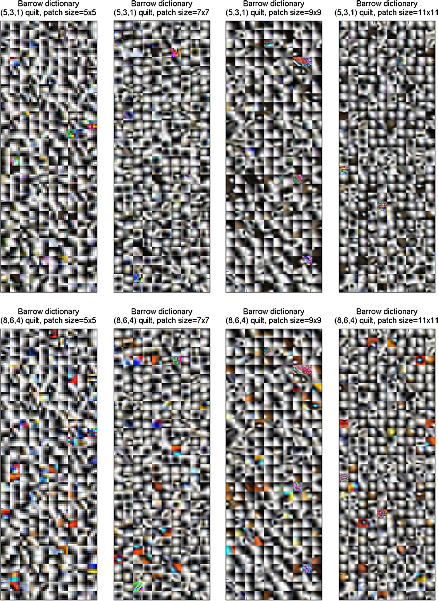

Each dictionary element is shown in the same position on the respective quilt for the two band combinations. Upon visual inspection, almost all the elements exhibit texture (i.e., variability in pixel intensity), and many contain oriented edges. We note that some of the elements that appear more uniform or more muted in one band combination exhibit more texture or intensity in the other band combination; that is, dictionary elements are sensitive to both spatial and spectral information. The Barrow dictionaries have features with sharp boundaries, i.e., high contrasts between two adjacent smooth features. This is consistent with the larger degree of geomorphic texture present in the Barrow image.

3.3.

Index Learned Dictionaries

We used the four normalized difference index images defined in Sec. 2.2 as the training data for our dictionaries. Specifically, the eight original WorldView-2 bands were replaced with the four corresponding index bands: NDVI, NDWI, NDSI, and NHFD. The data dimensionality is, thus, reduced by a factor of 2, which is helpful in reducing computational overhead. Additionally, as seen in Fig. 5, the type of discriminative features contained in the index bands can potentially steer the learning, by increasing separation in the training data between moisture content and vegetation (NDVI and NDWI), and diminishing the impact of soils on the other (NDSI). We again learn dictionaries for the patch sizes of $5 \times 5$ , $7 \times 7$ , $9 \times 9$ , and $11 \times 11$ , but this time reduce their dimensionality by a factor of two, resulting in number of elements $K = 150$ ; we show the resulting dictionary quilts in Fig. 7 in an (NDVI, NDWI, NDSI) band combination to highlight the spatial texture captured by these index dictionaries.

Fig. 7

Quilts of dictionary elements learned from Barrow normalized difference indices, for pixel patches of spatial extent $5 \times 5$ (first column), $7 \times 7$ (second column), $9 \times 9$ (third column), and $11 \times 11$ (fourth column). All dictionaries have $K = 150$ elements; each of the small squares in a quilt represents a dictionary element. Here we show an (NDVI, NDWI, NDSI) band combination to highlight spatial texture.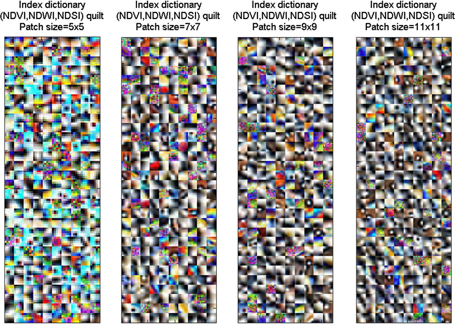

4. Clustering of Sparse Approximations

The CoSA algorithm seeks to automatically identify land cover categories in an unsupervised fashion. A $k$ -means clustering algorithm is used on undercomplete approximations of image patches (i.e., feature vectors), which in turn were found using the learned dictionaries. The main steps of the CoSA algorithm are summarized in Ref. 24, and some initial results on Barrow image data were shown in Refs. 23 and 25. Since we have two types of learned dictionaries, extracted from multispectral and index band data, each with four different spatial resolutions, we have a large number of clustering scenarios to consider. One important step is determining the number of clusters necessary for good classification, from a domain expert point of view. In this work, a range of fixed number of cluster centers, ${4, 8, 10, 12, 15, 20, 25, 30}$ , is considered for each of the four spatial resolutions, and few millions of multispectral patches randomly drawn from the training area are used to learn the cluster centers. The cluster training performance is evaluated as detailed in Ref. 31, from a quantitative (minimum distance convergence), as well as a qualitative (meaningful grouping of land cover features) standpoint. The trained cluster centers are used to generate land cover labels at the same spatial pixel resolution of the original satellite image. Specifically, for every pixel in the image, a clustering classification label is given based on its surrounding context (i.e., pixel patch centered on the respective pixel). In other words, we use a step-size of 1 pixel to extract overlapping patches for classification and do not extend image borders.

In an ideal case, performance in classification of land cover would be best optimized and/or evaluated based on domain expert verified pixel-level ground truth. The amount of such training and validation data would have to be relatively large considering the dimensionality of the satellite imagery, the complexity of the terrain, and the parameter space of the CoSA algorithm, e.g., of the order of thousands up to tens of thousands pixels (at the equivalent WorldView2 resolution). This could be an opportunity for field ecologists to generate such verified ground truth data. Meanwhile, in the absence of pixel-level ground truth, one way to assess the quality of the full image land cover labels generated by CoSA is to quantify their resulting intracluster distances. Table 2 details average intracluster distances for CoSA labels using both types of learned dictionaries, for the example case of $7 \times 7 pixel$ spatial resolution and the range of cluster centers considered. The mean and standard deviation of the intracluster distance after full image clustering are indicative of the degree of fit between the derived cluster centers and the true distribution of data, and so we desire both small mean intracluster distance, as well as small standard deviation within the cluster. At the selected pixel patch size in Table 2, both dictionary types lead to minimum mean intracluster distances at 20 cluster centers (bold values in Table 2), and the associated standard deviation is minimum in the multispectral dictionary case and the second smallest in the index dictionary case. Figure 8 summarizes the intracluster distances for all the four spatial resolutions and for both dictionary types.

Table 2

Mean intracluster distances after applying clustering of sparse approximations to the entire image for pixel patch size 7×7. For both dictionary types, minimum mean intracluster distances are obtained for 20 clusters (bold values).

Dictionary type	Number of cluster centers
Dictionary type	4	8	10	12	15	20	25	30
Multispectral learning	$0.365 \pm 0.224$	$0.995 \pm 0.547$	$1.090 \pm 0.507$	$0.753 \pm 0.369$	$1.330 \pm 0.431$	$0.127 \pm 0.099$	$1.279 \pm 0.383$	$0.194 \pm 0.112$
Index learning	$1.733 \pm 0.262$	$0.392 \pm 0.210$	$0.361 \pm 0.169$	$0.406 \pm 0.150$	$1.870 \pm 0.219$	$0.272 \pm 0.153$	$1.379 \pm 0.369$	$1.732 \pm 0.182$

Fig. 8

Mean intracluster distances after applying clustering of sparse approximations to the entire image using approximations derived with multispectral dictionaries (a) and with index dictionaries (b), for the four pixel patch sizes. Shown are mean value and corresponding standard deviation for every number of cluster centers considered.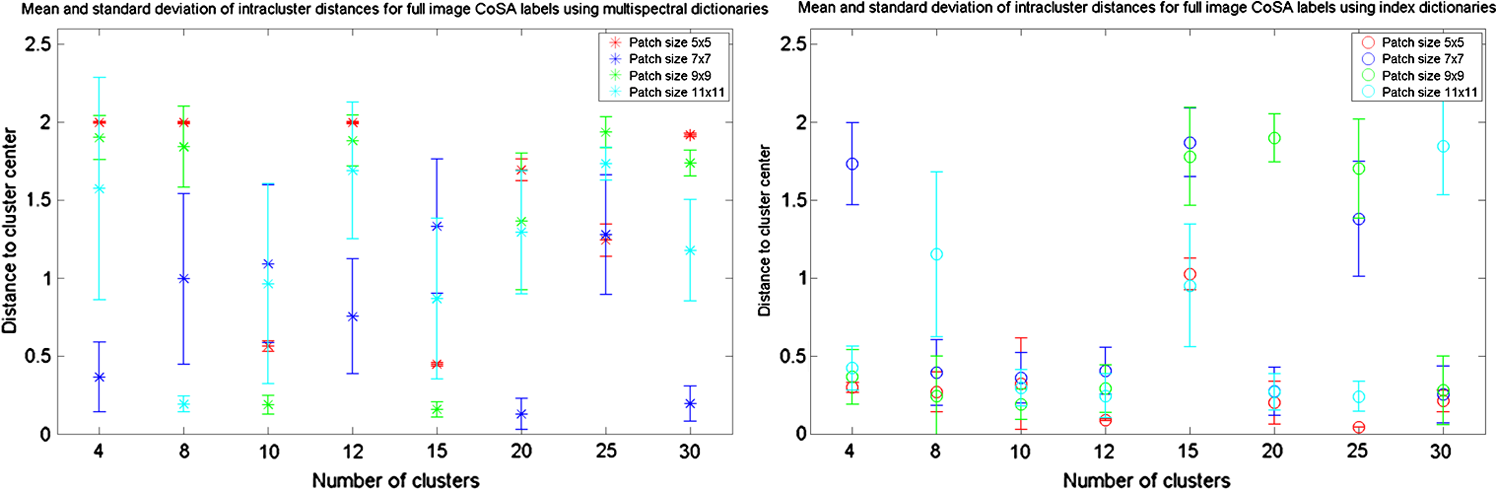

The left panel of Fig. 8 shows a wide range of clustering performance for approximations derived with dictionaries learned from raw multispectral data. For each spatial resolution, the corresponding minimum intracluster distance is reached with different numbers of cluster centers, and the standard deviations follow inconsistent patterns. A number of factors likely contribute to this effect, such as the spatial heterogeneity of the landscape, patch size, dictionary learning algorithm and convergence, and, last but not least, the $k$ -means clustering convergence. While it is very difficult to quantitatively evaluate how each factor impacts performance, the left panel of Fig. 8 suggests that some form of data regularization might be beneficial. Assuming that transformation of the original eight-band image into four derived band difference indices achieves some degree of desired regularization; the right side of Fig. 8 shows improved and more consistent cluster label quality, from a mathematical intracluster distance point of view. With few exceptions, mean and standard deviation of intracluster distances remain consistently small for a range of patch sizes and various number of cluster centers. We can only speculate that the few instances of higher intracluster distance are likely due to the local optimums chosen by the $k$ -means algorithm. A different clustering algorithm, such as expectation-maximization,³⁵ or a contiguous $k$ -means,³⁶ might lead to more consistent performance.

The final selection of the appropriate number of clusters for each image and at every resolution is based on analysis of CoSA results by an environmental domain expert. The expectation is that CoSA would segment the image into categories that preserve the features and structures visible in the WorldView-2 imagery, and do so better than the unsupervised classification on raw pixels illustrated in Figs. 3 and 4. We focus on analysis with 20 cluster centers (rectangular markups in Fig. 8) and explore the corresponding full image CoSA labels. Figure 9 shows these example clustering results for spatial resolutions of $5 \times 5$ [Fig. 9(a)], $7 \times 7$ [Fig. 9(b)], $9 \times 9$ [Fig. 9(c)], and $11 \times 11$ [Fig. 9(d)] for multispectral learned dictionaries, and Fig. 10 similarly shows results for the index learned dictionaries for the four pixel patch sizes.

Fig. 9

Category labels for Barrow image data using 20 clusters trained on approximations obtained with dictionaries learned from multispectral data for (a) $5 \times 5$ , (b) $7 \times 7$ , (c) $9 \times 9$ , and (d) $11 \times 11$ spatial resolution.

Fig. 10

Category labels for Barrow image data using 20 clusters trained on approximations obtained with dictionaries learned from index data for (a) $5 \times 5$ , (b) $7 \times 7$ , (c) $9 \times 9$ , and (d) $11 \times 11$ spatial resolution.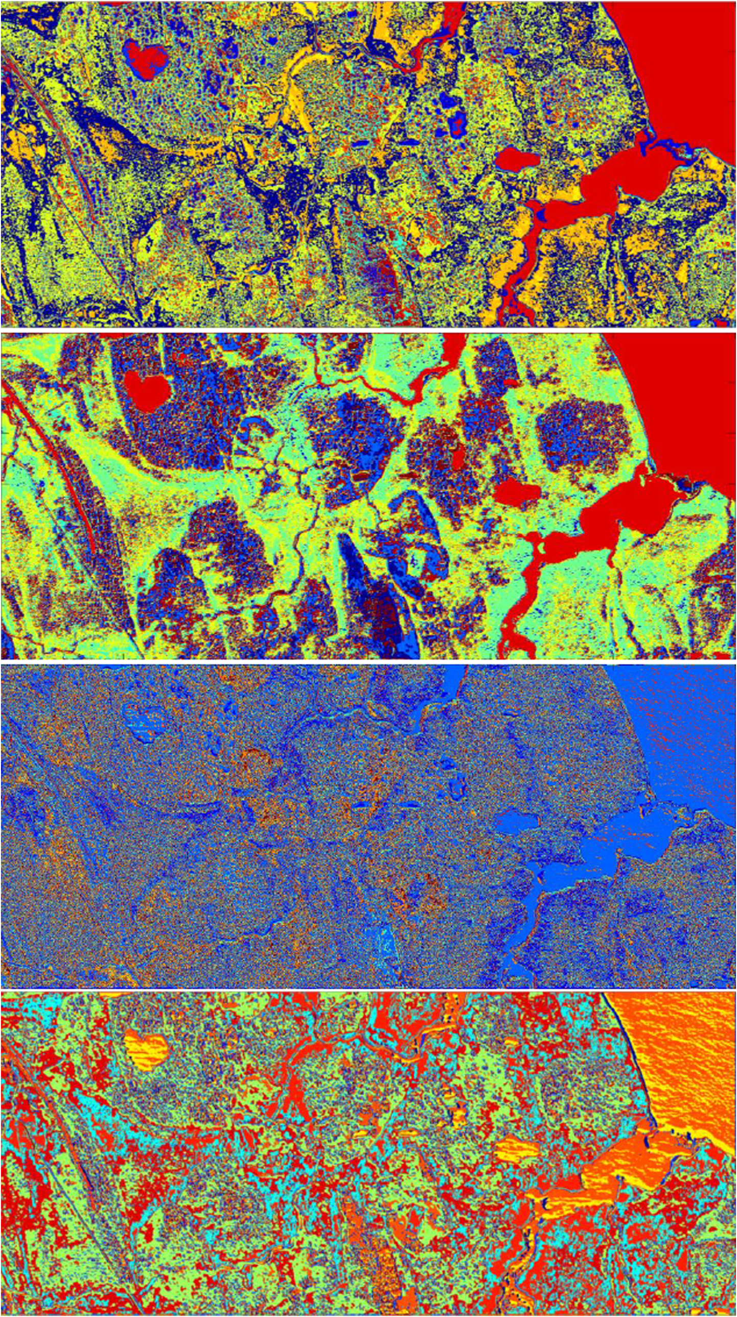

In the case of multispectral learned dictionaries, based on Fig. 8(a) we expect the most meaningful clustering to occur at $7 \times 7$ spatial resolution; we expect similar performances for patch sizes $9 \times 9$ and $11 \times 11$ ; we anticipate the poorest performance at $5 \times 5$ resolution. Indeed, if we consider the case of $9 \times 9$ patch size, we see a lot of label texture in the CoSA analysis [Fig. 9(c)]. The cluster labels seem to capture variations in turbidity levels in water bodies, when compared to the RGB image in Fig. 2, both in the lakes, as well as in the bay inlets. This sensitivity to moisture is also evident in the land cover clustering. The dark red labels map to high moisture content areas, such as low centered polygons and the snow drift on the left side of the image, and the blue labels correspond to dry areas, typically high centered polygons. When the dictionary spatial resolution is decreased to $7 \times 7 pixels$ [Fig. 9(b)] the clustering appears to capture the most meaningful land cover associations. In this case, water turbidity and moisture are no longer as prevalent in the clustering, and the learning and clustering are more dominated by information present in other spectral bands (i.e., vegetation sensitive bands). The light and dark blue labels now correspond to low centered polygonal ground, and the yellows and oranges to high centered polygons and the associated vegetation (grasses and shrubs). We can observe structure related to surface soil and vegetative cover, and see some texture directly correlating with polygonal ground.

In the case of dictionaries learned from normalized band difference indices, Fig. 8(b) indicates improved clustering performance should be expected for all spatial resolutions at 20 cluster centers, with the exception of the $9 \times 9$ case, in terms of intracluster mean distance. Visually, the labels in Fig. 10, indeed, show improved results at the expected resolutions, and for the $9 \times 9$ case, we see less correlation between labels and structures in the actual image. The CoSA analysis results in much more contiguous blocks for the 5, 7, and 11 patch sizes, and we observe more meaningful correspondence to land cover (surface soils and vegetation) and geomorphic texture (polygons) when compared to Fig. 2. The improvement in the case of $5 \times 5$ spatial resolution [Figs. 9(a) and 10(a)] is especially encouraging, as pixel patches of small spatial extend are desirable to reduce edge effects in the CoSA labels, i.e., label blurring. In particular for the Barrow area, exact label location is needed for polygonal ground structures and shoreline features, in order to evaluate and monitor moisture and soil changes.

4.1.

Separability of Classes Metric

A quantitative and meaningful metric for clustering can be derived based on intrinsic data properties, specifically by assessing how individual clusters capture normalized difference index information. For each pixel in a given cluster, we extract the values corresponding to its four normalized difference band indices detailed in Sec. 2.2. Effectively, we can now represent each cluster resulting from CoSA in this four-dimensional space defined by (NDVI, NDWI, NDSI, NHFD). We choose the three dominant indices, NDVI, NDWI, and NHFD, to visualize the clusters. Figure 11 shows cluster content scatter plots for 20 cluster centers at two spatial resolutions, $5 \times 5$ (left) and $7 \times 7$ (right), based on the associated CoSA performance illustrated in Figs. 9(a), 9(b), 10(a), and 10(b). We consider again the case of dictionaries learned from multispectral data (top) and index data (bottom).

Fig. 11

Scatter plots of clusters as a function of respective mean difference index values; diameter of spheres is proportional to intracluster mean variance across the three indices.

Each sphere in the scatter plots of Fig. 11 represents one cluster, plotted at coordinates given by the respective mean difference index values and of diameter proportional to the intracluster mean variance across the three indices. We see clusters are more separated (i.e., better class separation) and have more uniform variance distribution in the case of dictionaries learned from difference index bands, compared to dictionaries learned from multispectral data. It is worth noting that in the case of $7 \times 7 pixel$ patch size, Fig. 11 captures the performance improvement between the two dictionary types much stronger than the error bar plots of Fig. 8, which did not show drastic performance change at this resolution in the 20 cluster case.

Figure 11 suggests that a more natural metric for estimating cluster convergence may be one based on normalized band difference information, rather than Euclidian or cosine angle distance on raw pixel data. This will be explored in more detail in future work. The Barrow data provide some very useful insight into how landscape heterogeneity impacts the learning and clustering processes. Figures 9 and 10 illustrate how different landscape features are predominantly learned and classified at each dictionary spatial resolution, and how preprocessing band data prior to learning can help reduce label texture. This implies that the CoSA technique can be a viable multiscale/multiresolution analysis tool. At the same time, this wide range of possible CoSA label outcomes makes it difficult to apply directly to new data without a human in the loop. The exact purpose of the domain expert must inform the algorithm choices, for example, wide-area vegetative cover studies might require a larger pixel patch size, while geomorphic studies of polygonal ground, for example, might require a smaller patch size. One must also account for any potential edge effects introduced by using patch sizes that are too large. And last, but not least, information extraction from a satellite image is in a broad sense highly dependent on the native pixel resolution, and additional issues, such as spectral unmixing, would have to be addressed for lower-resolution images, e.g., Landsat data. The challenge, therefore, to making the CoSA method successful for classification in remote sensing will be understanding how to precondition the learning toward features of interest.

4.2.

Aspects of CoSA Implementation and Software Complexity

For most learned dictionary-based applications, there are two separate algorithm components that need to be separately optimized: the learning stage and the classification stage. Both stages have some algorithm sections that have low memory demands and are parallelizable, and some that are computationally intensive and sequential. For our specific data case of high-resolution multispectral imagery, the memory access demands are significant and must also be considered in the CoSA algorithm implementation. On the hardware side, we run CoSA using a multiprocessor (Intel Xeon X555) Windows 7 64-bit machine, with a total of 32 cores, and have the option to distribute computing across additional cores on our local cluster. We also were able to integrate the use of an Nvidia Tesla graphic processing unit (GPU) card.

Several implementation approaches were pursued, from all-CPU processing, to mostly GPU processing, to various combinations in between. Since a few components of the dictionary learning algorithm and matching pursuit search do not yet have a Compute Unified Device Architecture supported implementation, full GPU computation was not possible. The challenge to implementing the CoSA algorithm, therefore, was to jointly optimize computation, memory access, and communication time between CPU and GPU. The final implementation decision was made based on fastest overall computational time and computational scalability with changes in image size, using MATLAB®’s Profiler. The satellite image to be processed is typically preloaded on the GPU and then partitioned into large blocks, of the order of tens of thousands of pixels, which are requested by the CPU as needed. The core of CoSA runs on CPUs and effectively uses the GPU only for fast access to preloaded images. The two separate CoSA algorithm components that need to be optimized are the learning stage and the classification stage.

The learning stage is computationally very expensive, depending on the chosen dictionary size and the amount of training data available. In our case, this is upfront computational overhead and can be reduced by the use of parallel computing hardware. At a particular sequential update iteration, we can scatter the $K$ inner products between data and dictionary elements across multiple cores, resulting in O(LNP) complexity, where $L$ is the sparsity factor, $N$ is the length of a dictionary element, and $P$ is the number of training data windows. The Hebbian dictionary update grows linearly with the length of dictionary element (or size of data windows). During a learning iteration, the CPU will retrieve one image partition at a time, from which it will randomly select batches of training patches to update the dictionary. The cluster centers are learned in a similar fashion on the CPU, by iterating over randomly drawn large batches of image patches (tens of thousands). The total learning stage computational time is of the order of hours, varying from $\sim 3 h$ up to $\sim 16$ , depending on the specific dictionary learning setup, i.e., number of elements, convergence criteria, learning rate, size of training set, batch size, patch size, type (index or raw).

In the classification stage, the labeling of the entire image data into land cover categories is done using a parallel, vectorized implementation. Since our learned dictionaries are typically undercomplete, i.e., $K ≪ N$ , the search space for estimating sparse approximations for image patches is reduced, leading to some increase in classification speed. The image partitions are processed in parallel across multiple CPU cores. Every partition is buffered prior to CoSA processing, that is, every image patch is reshaped in the associated 1-D vector and the resulting matrix of thousands of rows is processed at the same time, lowering the communication time and achieving further improvement from the algorithmic vectorization. Land cover labeling of a partition takes, on average, 165.16 s, resulting in an average of 24.77 min for the Barrow data at $3 \times 3$ partitions.

5. Conclusion

This paper presents an extension of learned dictionary techniques to unsupervised classification of land cover in multispectral satellite imagery, using CoSA. We show a new dictionary learning approach based on normalized difference indices, as well as direct learning from multispectral data. We also explore a quantitative metric based on normalized band differencing to evaluate spectral properties of the clusters, in order to potentially aid in assigning land cover categories to the cluster labels. The clustering appears to detect real variability, but some of the associations it makes could be grouped or are not important for one type of classification versus another (e.g., vegetative versus hydrologic studies). A potential CoSA multiscale approach could be successful in developing a classification scheme that shows vegetation at one scale and topographic features at another. The end goal of this work is to use CoSA for detecting yearly and seasonal changes in land cover and soil moisture, which is needed for climate change monitoring over wide areas in the Arctic. The CoSA derived land cover labels, therefore, need to be correlated by an environmental scientist to actual landscape features, be those vegetative, hydrologic, or geomorphic, and this is the topic of current investigation. Additionally, we are exploring how to learn dictionaries and clusters to be scalable to images from the same region in different seasons, and use them for change detection.

Acknowledgments

This work was supported by the U.S. Department of Energy (DOE) through the LANL/LDRD Program. Application of the methodology and continued development is supported by DOE’s Office of Science, Biological and Environmental Research (BER) Program, through the Next Generation Ecosystem Experiment (NGEE)—Arctic project.

References

1.

S. P. Brumbyet al., “Large-scale functional models of visual cortex for remote sensing,” in 38th IEEE Applied Imagery Pattern Recognition, Vision: Humans, Animals, and Machines, 1 –6 (2009). Google Scholar

2.

Arctic Climate Impact Assessment, Cambridge University Press, New York (2005). Google Scholar

3.

M. Sturmet al., “Snow-shrub interactions in Arctic tundra: a hypothesis with climatic implications,” J. Clim., 14 (3), 336 –344 (2001). http://dx.doi.org/10.1175/1520-0442(2001)014<0336:SSIIAT>2.0.CO;2 JLCLEL 0894-8755 Google Scholar

4.

C. R. BurnS. V. Kokelj, “The environment and permafrost of the Mackenzie delta area,” Permafr. Periglac. Processes, 20 (2), 83 –105 (2009). http://dx.doi.org/10.1002/(ISSN)1099-1530 PEPPED 1099-1530 Google Scholar

5.

P. Marshet al., “Snowmelt energetics at a shrub tundra site in the western Canadian Arctic,” Hydrol. Processes, 24 (25), 3603 –3620 (2010). http://dx.doi.org/10.1002/hyp.v24:25 HYPRE3 1099-1085 Google Scholar

6.

T. C. LantzS. E. GergelG. H. R. Henry, “Response of green alder (Alnus viridis subsp fruticosa) patch dynamics and plant community composition to fire and regional temperature in north-western Canada,” J. Biogeogr., 37 (8), 1597 –1610 (2010). http://dx.doi.org/10.1111/j.1365-2699.2010.02317.x JBIODN 1365-2699 Google Scholar

7.

T. C. LantzS. E. GergelS. V. Kokelj, “Spatial heterogeneity in the shrub tundra ecotone in the Mackenzie delta region, Northwest territories: implications for Arctic environmental change,” Ecosystems, 13 (2), 194 –204 (2010). http://dx.doi.org/10.1007/s10021-009-9310-0 ECOSFJ 1432-9840 Google Scholar

8.

I. Olthofet al., “Recent (1986–2006) vegetation-specific NDVI trends in northern Canada from satellite data,” Arctic, 61 (4), 381 –394 (2008). http://dx.doi.org/10.14430/arctic46 ATICAB 0004-0843 Google Scholar

9.

M. D. Walkeret al., “Plant community responses to experimental warming across the tundra biome,” Proc. Natl. Acad. Sci. U S A, 103 (5), 1342 –1346 (2006). http://dx.doi.org/10.1073/pnas.0503198103 PNASA6 0027-8424 Google Scholar

10.

C. GangodagamageP. BelmontE. Foufoula-Georgiou, “Revisiting scaling laws in river basins: new considerations across hillslope and fluvial regimes,” Water Res. Res., 47 (7), W07508 (2011). http://dx.doi.org/10.1029/2010WR009252 WRERAQ 0043-1397 Google Scholar

11.

H. E. Epsteinet al., “Detecting changes in arctic tundra plant communities in response to warming over decadal time scales,” Glob. Change Biol., 10 (8), 1325 –1334 (2004). http://dx.doi.org/10.1111/gcb.2004.10.issue-8 1354-1013 Google Scholar

12.

D. A. Stowet al., “Remote sensing of vegetation and land-cover change in Arctic tundra ecosystems,” Remote Sens. Environ., 89 (3), 281 –308 (2004). http://dx.doi.org/10.1016/j.rse.2003.10.018 RSEEA7 0034-4257 Google Scholar

13.

F. Costardet al., “Impact of the global warming on the fluvial thermal erosion over the Lena river in Central Siberia,” Geophys. Res. Lett., 34 (14), L14501 (2007). http://dx.doi.org/10.1029/2007GL030212 GPRLAJ 0094-8276 Google Scholar

14.

J. C. MarsD. W. Houseknecht, “Quantitative remote sensing study indicates doubling of coastal erosion rate in past 50 yr along a segment of the Arctic coast of Alaska,” Geology, 35 (7), 583 –586 (2007). http://dx.doi.org/10.1130/G23672A.1 GLGYBA 0091-7613 Google Scholar

15.

M. Chenet al., “Temporal and spatial pattern of thermokarst lake area changes at Yukon Flats, Alaska,” Hydrol. Processes, 28 (3), 837 –852 (2014). http://dx.doi.org/10.1002/hyp.v28.3 HYPRE3 1099-1085 Google Scholar

16.

G. Hugeliuset al., “High-resolution mapping of ecosystem carbon storage and potential effects of permafrost thaw in periglacial terrain, European Russian Arctic,” J. Geophys. Res. Biogeosci., 116 (G3), G03024 (2011). http://dx.doi.org/10.1029/2010JG001606 Google Scholar

17.

R. B. Myneniet al., “The interpretation of spectral vegetation indexes,” IEEE Trans. Geosci. Remote Sens., 33 (2), 481 –486 (1995). http://dx.doi.org/10.1109/36.377948 IGRSD2 0196-2892 Google Scholar

18.

S. P. Brumbyet al., “Evolving feature extraction algorithms for hyperspectral and fused imagery,” in Proc. of the Fifth Int. Conf. on Information Fusion, 986 –993 (2002). Google Scholar

19.

N. R. Harveyet al., “Parallel evolution of image processing tools for multispectral imagery,” Proc. SPIE, 4132 72 –82 (2000). http://dx.doi.org/10.1117/12.406611 PSISDG 0277-786X Google Scholar

20.

N. R. Harveyet al., “Automated simultaneous multiple feature classification of MTI data,” Proc. SPIE, 4725 346 –356 (2002). http://dx.doi.org/10.1117/12.478767 PSISDG 0277-786X Google Scholar

21.

N. R. Harveyet al., “Comparison of GENIE and conventional supervised classifiers for multispectral image feature extraction,” IEEE Trans. Geosci. Remote Sens., 40 (2), 393 –404 (2002). http://dx.doi.org/10.1109/36.992801 IGRSD2 0196-2892 Google Scholar

22.

N. R. Harveyet al., “Finding golf courses: the ultra high tech approach,” Lec. Notes Comput. Sci., 1803 54 –64 (2000). http://dx.doi.org/10.1007/3-540-45561-2 LNCSD9 0302-9743 Google Scholar

23.

D. I. Moodyet al., “Undercomplete learned dictionaries for land cover classification in multispectral imagery of Arctic landscapes using CoSA: clustering of sparse approximations,” Proc. SPIE, 8743 87430B (2013). http://dx.doi.org/10.1117/12.2016135 PSISDG 0277-786X Google Scholar

24.

D. I. Moodyet al., “Unsupervised land cover classification in multispectral imagery with sparse representations on learned dictionaries,” in IEEE Applied Imagery Pattern Recognition Workshop, Computer Vision: Time for Change, 1 –10 (2012). Google Scholar

25.

D. I. Moodyet al., “Land cover classification in multispectral satellite imagery using sparse approximations on learned dictionaries,” Proc. SPIE, 9124 91240Y (2014). http://dx.doi.org/10.1117/12.2049843 PSISDG 0277-786X Google Scholar

26.

DigitalGlobe®, “The benefits of the 8 spectral bands of WorldView,” (2012) https://www.digitalglobe.com/sites/default/files/DG-8SPECTRAL-WP_0.pdf ( January ). 2012). Google Scholar

27.

S. S. Hubbardet al., “Quantifying and relating land-surface and subsurface variability in permafrost environments using LiDAR and surface geophysical datasets,” Hydrogeol. J., 21 (1), 149 –169 (2013). http://dx.doi.org/10.1007/s10040-012-0939-y HJYOAW 1431-2174 Google Scholar

28.

K. M. Hinkelet al., “Spatial extent, age, and carbon stocks in drained thaw lake basins on the Barrow Peninsula, Alaska,” Arct. Antarct. Alp. Res., 35 (3), 291 –300 (2003). http://dx.doi.org/10.1657/1523-0430(2003)035[0291:SEAACS]2.0.CO;2 1523-0430 Google Scholar

29.

S. D. Wullschlegeret al., “Plant community composition and nitrogen stocks across complex polygonal landscapes on the North Slope of Alaska,” in AGU Fall Meeting, (2013). Google Scholar

30.

A. F. Wolf, “Using Worldview-2 Vis-NIR multispectral imagery to support land mapping and feature extraction using normalized difference index ratios,” Proc. SPIE, 8390 83900N (2012). http://dx.doi.org/10.1117/12.917717 PSISDG 0277-786X Google Scholar

31.

D. I. Moodyet al., “Learning sparse discriminative representations for land cover classification in the Arctic,” Proc. SPIE, 8514 85140Q (2012). http://dx.doi.org/10.1117/12.930182 PSISDG 0277-786X Google Scholar

32.

S. G. MallatZ. Zhang, “Matching pursuits with time-frequency dictionaries,” IEEE Trans. Signal Process., 41 (12), 3397 –3415 (1993). http://dx.doi.org/10.1109/78.258082 ITPRED 1053-587X Google Scholar

33.

T. BlumensathM. E. Davies, “Gradient pursuits,” IEEE Trans. Signal Process., 56 (6), 2370 –2382 (2008). http://dx.doi.org/10.1109/TSP.2007.916124 ITPRED 1053-587X Google Scholar

34.

S. S. B. ChenD. L. DonohoM. A. Saunders, “Atomic decomposition by basis pursuit,” SIAM Rev., 43 (1), 129 –159 (2001). http://dx.doi.org/10.1137/S003614450037906X SIREAD 0036-1445 Google Scholar

35.

C. F. J. Wu, “On the convergence properties of the EM algorithm,” Ann. Stat., 11 (1), 95 –103 (1983). http://dx.doi.org/10.1214/aos/1176346060 ASTSC7 0090-5364 Google Scholar

36.

J. TheilerG. Gisler, “A contiguity-enhanced k-means clustering algorithm for unsupervised multispectral image segmentation,” Proc. SPIE, 3159 108 –118 (1997). http://dx.doi.org/10.1117/12.279444 PSISDG 0277-786X Google Scholar

Biography

Daniela I. Moody is a scientist on the Machine Learning and Data Exploitation Team in LANL’s ISR-3 Data Space Systems Group. She received her PhD degree in electrical engineering from the University of Maryland, College Park, in 2012 and has been at LANL since 2006. Her current work focuses on developing improved feature extraction algorithms that combine adaptive signal processing with compressive sensing, and with machine learning techniques. She is applying such algorithms to a wide range of datasets, including satellite-sensed RF data, multispectral imagery, and imaging surveys. She is a member of SPIE and IEEE.

Steven P. Brumby is a senior research scientist at Los Alamos National Laboratory, Information Sciences Group, working on development of novel sparse-coding and deep-learning algorithms for video, image and signals analysis. He received his PhD degree in theoretical physics at the University of Melbourne (Australia) in 1997. He is a coinventor of LANL’s GENIE image analysis algorithm (R&D Award 2002). He is a principal investigator of LANL’s Video Analysis and Search Technology (VAST) project.

Joel C. Rowland is a staff scientist in Los Alamos’ Earth and Environmental Sciences Division. He received his PhD degree in Earth and Planetary Science from the University of California, Berkeley in 2007. His research focuses on land surface dynamics in Arctic environments, in particular on how rivers and lakes in permafrost settings will respond to warming, permafrost loss and changes in hydrology. He is part of DOE’s Next Generation Ecosystem Experiment Arctic research project team.

Garrett L. Altmann is a graduate research assistant in the Environmental Sciences Division at Los Alamos National Laboratory. He specializes in GIS and remote sensing, with an interest in applying visualization techniques to communicate science. He received his BA degree in geography from UC Santa Barbara, and his MSc degree in natural resources management from the University of Alaska Fairbanks.

CC BY: © The Authors. Published by SPIE under a Creative Commons Attribution 4.0 Unported License. Distribution or reproduction of this work in whole or in part requires full attribution of the original publication, including its DOI.

Citation Download Citation

Daniela I. Moody, Steven P. Brumby, Joel C. Rowland, and Garrett L. Altmann "Land cover classification in multispectral imagery using clustering of sparse approximations over learned feature dictionaries," Journal of Applied Remote Sensing 8(1), 084793 (9 December 2014). https://doi.org/10.1117/1.JRS.8.084793

Published: 9 December 2014

Access the abstract

JOURNAL ARTICLE
19 PAGES

DOWNLOAD PAPER SAVE TO MY LIBRARY

GET CITATION

CITATIONS

Cited by 15 scholarly publications.

Explore citations on Lens.org

KEYWORDS

Associative arrays

Image classification

Multispectral imaging

Spatial resolution

Satellites

Earth observing sensors

Satellite imaging

1.

Introduction

2.

Arctic Study Site