Two-dimensional sparse synthetic aperture radar imaging method with stepped-frequency waveform

Fufei Gu; Qun Zhang; Hao Lou; Zhi’an Li; Ying Luo

doi:10.1117/1.JRS.9.096099

7 January 2015 Two-dimensional sparse synthetic aperture radar imaging method with stepped-frequency waveform

Fufei Gu, Qun Zhang, Hao Lou, Zhi’an Li, Ying Luo

Author Affiliations +

Journal of Applied Remote Sensing, Vol. 9, Issue 1, 096099 (January 2015). https://doi.org/10.1117/1.JRS.9.096099

Abstract

Stepped-frequency waveforms (SFWs) can use the digital signal processing method to obtain high-range resolution with relatively narrow instantaneous bandwidth, which has been used in synthetic aperture radar (SAR). However, SFWs have the disadvantages of poor antijamming capability and a long period of transmission. Also, in the coherent integration time, some echo data are frequently lost. A two-dimensional sparse imaging method in the space and frequency domains for SAR is proposed based on compressed sensing (CS) theory. A sparse SFW for SAR imaging is formed and analyzed first, which has the advantages of better antijamming capability and a shorter time period of transmission. The range compression is completed by using CS theory. As to the sparse echo data in the space domain, the imaging operator and the CS-based imaging scheme are constructed to simultaneously implement the range cell migration correction and azimuth compression. Compared with the conventional SAR imaging method of SFWs, a much smaller number of frequencies and a smaller amount of imaging data are required for SAR imaging by using the proposed method. Finally, the effectiveness of the proposed method is proven by simulation and experimental results.

1. Introduction

Synthetic aperture radar (SAR) can realize imaging for the ground targets all day and under all weather conditions, and can achieve a high resolution in range direction due to the use of high transmitted-pulse bandwidth and in azimuth direction due to the storage of data over a certain observation time.¹^,² However, along with the improvement of range resolution, the bandwidth of the transmitted signal will increase sharply, which is a huge challenge for sampling at the receiver using analog-to-digital technology.³ Stepped-frequency waveforms (SFWs) consist of sequences of single-frequency pulses where the frequency of each pulse is increased by discrete steps.⁴^,⁵ Thus, SFWs are able to use the wide radio-frequency band of a frequency-agile radar with a narrow-band receiver which only needs simple hardware.⁶ Therefore, SFWs have been widely employed to increase system bandwidth. However, the frequency-stepped value of conventional SFWs is constant, and can be easily jammed. Meanwhile, SFWs are a group of subpulses which require a long time period of transmission and may result in Doppler ambiguity. These disadvantages dramatically reduce its applications.

In the last few years, the compressed sensing (CS) theory, which has been introduced in Refs. 7 and 8, indicates that one can stably and accurately reconstruct nearly sparse signals from dramatically undersampled data in an incoherent domain. With this prominent advantage, the CS theory has been used in wide-ranging applications. Meanwhile, the idea of CS has also been introduced in imaging radar system.⁹^–¹⁵ In Ref. 10, a CS-based radar imaging method is proposed in which the pulse compression matched filter is no longer needed. In Ref. 11, a random-frequency SAR imaging scheme based on CS is put forward. The advantage of this method is that only a small number of random frequencies are needed to reconstruct the image of the targets. However, it does not consider the situation that some of SAR echo data may be lost in the coherent integration time. In Ref. 12, the CS-based imaging algorithm is proposed to obtain the super-resolving imaging result with full data for stepped-frequency SAR. Also, the sparse recovery method is utilized to estimate the range and Doppler of multiple targets with random stepped-frequency radar.¹³ Reference 14 proposes a step-frequency radar system based on compressive sampling, which can use a smaller bandwidth to achieve a high range and speed resolution. If a part of the subpulses of SFWs is randomly selected for transmission, the interference frequency band will be avoided and the time period to transmit will be shortened,¹⁵ which can improve the antijamming capability, increase the equivalent pulse repetition frequency (PRF), and restrain the azimuth ambiguity. Thus, a sparse SFW for SAR imaging is studied in this paper.

In addition, it frequently occurs that some of SAR echo data are contaminated or lost in the coherent integration time. The contaminated data must be abandoned, which leads to the conventional SAR imaging method being invalid. Due to the transmitted signal is the sparse SFW, the SAR echo data are two-dimensional (2-D) sparsity both in the frequency and space domains. In this paper, a novel 2-D sparse SAR imaging method is put forward. First, after analyzing the imaging model with the sparse SFWs, the range compression is completed by using CS theory instead of the inverse discrete Fourier transform (IDFT) processing. Second, in azimuth imaging processing, the imaging operator is constructed by multiplying the diagonal 2-D decoupling frequency function by the azimuth compression function. Thus, the range cell migration correction and azimuth compression are implemented simultaneously by the CS-based imaging scheme. The main advantages of our method can be concluded as follows:

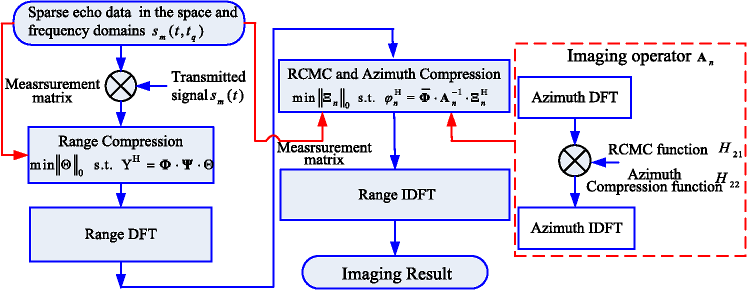
1. By using the sparse SFWs, the antijamming capability of the SAR imaging system is improved and PRF is increased, which can restrain the azimuth ambiguity.
2. Even if some of the echo data are contaminated or lost in the space domain, the range cell migration correction and azimuth compression can be achieved by constructing the imaging operator and the CS-based imaging scheme. In other words, we can obtain the SAR imaging result with small amounts of data, which is very important for high-resolution SAR imaging.

The organization of this paper is as follows. Section 2 analyzes the signal model for SAR imaging with sparse SFWs. Then, after introducing CS theory, range compression is completed by using CS theory in Sec. 3. In Sec. 4, the azimuth imaging method with the sparse echo data in the space domain is proposed by constructing an imaging operator and CS-based imaging scheme which can implement range cell migration correction and azimuth compression. Simulation and experimental results are presented in Sec. 5 to validate the effectiveness of the proposed approach. Finally, we make some conclusions in Sec. 6.

2. Signal Model for Synthetic Aperture Radar Imaging with Sparse Stepped Frequency

2.1.

Sparse Stepped-Frequency Waveforms

The SFW is a kind of synthesized bandwidth signals which can use a sequence of single-frequency pulses to achieve an ultrawide bandwidth, and the frequency of each pulse is increased in steps. The SFW can be expressed as

Eq. (1)

s_{n} (t) = u (t - n T_{p}) \exp (j 2 π (f_{0} + n Δ f) t + θ_{n}),

where

n = 1,2, \dots, N

,

N

is the number of pulses in one sequence,

u (t)

denotes a rectangular window,

T_{p}

is the window width (this also refers to the time duration of each pulse),

f_{0}

is the carrier frequency, and

Δ f

is the frequency-stepped size.

The sparse SFW is directly expanded from the full-band SFW: if only portions of full-band subpulses are transmitted, then a sparse SFW is formed, which can shorten the time period of transmission. For example, the processing interval is $N T_{p}$ when transmitting a full-band SFW for a burst, whereas the processing interval is $M T_{p}$ when $M (M < N)$ subpulses are transmitted for a burst. So the processing interval is reduced and the equivalent PRF is increased, thus the Doppler ambiguity can be restrained. Meanwhile, the sparse SFW cannot be interfered with by external radio-frequency sources. With the prior information of interferences, a sparse SFW radar system would be programmed to step over the frequency bands with interferences so that clean echo signals can be obtained.

To make the notation clear, the frequency-stepped value of sparse SFW is denoted by $f_{m} = n_{m} Δ f$ , where $n_{m}$ is a subset of $[1 : N]$ , and $m$ runs from 1 to $M$ . The $m$ ’th subpulse in a burst of sparse SFW can be expressed as

Eq. (2)

s_{m} (t) = u (t - m T_{p}) \exp (j 2 π (f_{0} + n_{m} Δ f) t + θ_{m}) .

The sparsity level of sparse SFW is defined as

Eq. (3)

γ = \frac{N - M}{N} .

In the following section, the SAR imaging model is analyzed by this sparse SFW.

2.2.

Synthetic Aperture Radar Imaging Model with Sparse Stepped-Frequency Waveforms

The geometric model for SAR imaging with sparse SFWs is shown in Fig. 1. The SAR system adopts the “stop-and-go” model. The imaging scene is modeled by using the point-scattering model, which includes $I$ scatterers with the scattering coefficients $σ_{i}$ , $i = 1,2, \dots, I$ .

Fig. 1

Geometric model for synthetic aperture radar (SAR) imaging with sparse stepped-frequency waveforms (SFWs). $P_{i}$ denotes the $i$ ’th scatter point and its coordinate is $(x_{i}, y_{i}, 0)$ . $P_{0}$ is the center of the observed scene and its coordinate is $(x_{0}, y_{0}, 0)$ . $R_{0}$ and $R_{i}$ are the distances of $P_{0}$ and $P_{i}$ to the air route, respectively.

Assuming that the radar system transmits sparse SFW, the expression of $m$ ’th subpulse in a burst of sparse SFW is shown in Eq. (2). Thus, the received echoes can be expressed as

Eq. (4)

s_{m} (t, t_{q}) = \sum_{i = 1}^{I} σ_{i} u (t - m T_{p} - 2 R_{i} (t_{q}) / c) \exp (j 2 π (f_{0} + n_{m} Δ f) (t - 2 R_{i} (t_{q}) / c) + θ_{m}),

where

t

denotes the fast time,

t_{q}

denotes the slow time,

c

is the propagation speed of electromagnetic wave, and

R_{i} (t_{q})

is the distance of the

i

’th scatter point to radar at

t_{q}

. From the geometry model for SAR imaging as shown in Fig. 1,

R_{i} (t_{q})

can be obtained easily:

Eq. (5)

R_{i} (t_{q}) = \sqrt{{(v t_{q} - x_{i})}^{2} + h^{2} + y_{i}^{2} + x_{i}^{2}} = \sqrt{{(v t_{q} - x_{i})}^{2} + R_{i}^{2}} .

We use the local oscillator signal with a frequency of $f_{0} + n_{m} Δ f$ as the reference signal to demodulate the received echo $s_{m} (t, t_{q})$ . The demodulation process can be written as

Eq. (6)

s_{cm} (t, t_{q}) = s_{m} (t, t_{q}) \cdot s_{m}^{*} (t) = \sum_{i = 1}^{I} σ_{i} u (t - m T_{p} - 2 R_{i} (t_{q}) / c) \exp (- j 4 π (f_{0} + n_{m} Δ f) R_{i} (t_{q}) / c),

where

s_{cm} (t, t_{q})

is the demodulated baseband signal. Sampling is performed after demodulation of the received echo. In order to obtain the maximum amplitude of the echo signal, the echo signal should be sampled at the center of the subpulse. The sampling time

t_{m}

should be¹⁴

Eq. (7)

t_{m} = m T_{p} + \frac{T_{p}}{2} + \frac{2 R^{'}}{c},

where

R^{'}

is the distance between the radar and the center of the imaging scene. The extracted data are

Eq. (8)

s_{c m} (t_{q}) = \sum_{i = 1}^{I} σ_{i} \exp (- j 4 π (f_{0} + n_{m} Δ f) R_{i} (t_{q}) / c) = \sum_{i = 1}^{I} σ_{i} \cdot \exp (- j 4 π n_{m} Δ f R_{i} (t_{q}) / c) \cdot \exp (- j 4 π f_{0} R_{i} (t_{q}) / c) .

It should be noted that the demodulated signal $s_{cm} (t_{q})$ consisted of two phase terms, the first term of which is linearly related to $n_{m}$ for a fixed $R_{i} (t_{q})$ . According to Refs. 14 and 16, if the transmitted signal is full-band SFW, i.e., ${n_{m}}$ is uniform, then the range compression can be completed by performing IDFT about $n_{m}$ . However, in the case of sparse SFW, conventional methods for range compression would generate high side-lobes and grating lobes, which can contaminate the range profiles. Thus, a novel range compression method should be presented.

3. Range Imaging with Sparse Stepped-Frequency Waveforms

3.1.

Compressed Sensing Theory

Let $h \in R^{N_{1}}$ denotes a finite signal of interest. If there exists a basis matrix $Ψ = {ψ_{1}, ψ_{2}, \dots, ψ_{N_{1}}}$ satisfying $h = Ψ Θ$ , where $Θ = {θ_{i}}$ is a $K$ -sparse vector (namely it can be approximated by its $K$ largest coefficients or its coefficients following a power decay law with $K$ strongest coefficients¹⁷), then $h$ can be reduced from $N_{1}$ -dimension to $M_{1}$ -dimension { $M_{1} \geq O (K \log (N_{1}))$ ⁷}, which is expressed as

Eq. (9)

u^{M_{1} \times 1} = Φ^{M_{1} \times N_{1}} h^{N_{1} \times 1} = Φ^{M_{1} \times N_{1}} Ψ^{N_{1} \times N_{1}} Θ^{N_{1} \times 1},

where

Φ

denotes a measurement matrix and

u

is the measurements’ vector of signal

h

. Generally, recovery of signal

h

from the measurements

u

is an ill-posed problem because of

M_{1} ≪ N_{1}

. However, the CS theory tells us that when the matrix

Φ Ψ

has the restricted isometry property (RIP),⁸ then it is possible to recover the

K

largest coefficients from the measurements

u

. The RIP is a requirement for the convergence of the reconstruction algorithm, and a detailed expression is given as follows:

Eq. (10)

1 - ε_{K} \leq \frac{{‖ Φ Ψ Θ ‖}_{2}}{{‖ Θ ‖}_{2}} \leq 1 + ε_{K}, (ε_{K} > 0) .

When the RIP holds, the coefficients ${θ_{i}}$ of signal $h$ can be accurately reconstructed from measurements $u$ . It is difficult to directly validate a measurement matrix satisfying the RIP constraints given in Ref. 18, but fortunately, the RIP is closely related to an incoherency between $Φ$ and $Ψ$ , where the rows of $Φ$ do not provide a sparse representation of the columns of $Ψ$ and vice versa. When $Φ Ψ$ satisfies the RIP constraints, the coefficients ${θ_{i}}$ of signal $h$ can be reconstructed by solving the following optimization problem:

Eq. (11)

\min {‖ Θ ‖}_{0} subject to u = Φ Ψ Θ,

where

{‖ \cdot ‖}_{0}

denotes

l_{0}

norm, and min(.) denotes the minimization. How to solve this optimization problem is an important aspect of CS theory. Due to the discontinuousness of

l_{0}

norm, it is difficult to solve Eq. (11) by a gradient method. The smoothed

l_{0}

(SL0) algorithm, which uses the continuous Gauss function to approach the

l_{0}

norm, is proposed in Ref. 19. It has a fast reconstruction speed and high-reconstruction accuracy. Therefore, the SL0 algorithm is adopted to solve the above optimization problem. In the case of a noisy observation, Eq. (11) can be rewritten as

Eq. (12)

\min ‖ Θ ‖_{0} subject to u = Φ Ψ Θ + n,

where

n

is the noise term.

Θ

can be obtained by

Eq. (13)

\hat{Θ} = \arg \min {‖ Θ ‖}_{0} subject to {‖ u - Φ Ψ Θ ‖}_{2} < ε,

where

ε = ‖ n ‖_{2}

is at the noise level. A good performance for the reconstruction of

Θ

is ensured when the signal-to-noise ratio (SNR) is relatively high. Setting a different parameter of

ε

, we can extract different amounts of

Θ

. However, if

ε

is large, the small value of

Θ

may be treated as noise and rejected, and if

ε

is small, the noise elements may distort

Θ

. Thus, the estimation of noise

ε

is essential. The Gaussian noise usually distributes evenly, and there are many range cells containing only noise. Given enough noise samples by those pure-noise cells, we can estimate

ε

with high accuracy.

Clearly, three elements are specified in CS theory: (1) a basis to support sparse representation of the signal; (2) a measurement operator to make the matrix $Φ Ψ$ have RIP; and (3) a reconstruction algorithm to solve the optimization problem.

3.2.

Range Compression Method

Assume that the transmitted signal is full-band SFW $s_{n} (t)$ . The echo signal of $s_{n} (t)$ is processed by Eqs. (6) and (8) in the aforementioned analysis, and $s_{cn} (t_{q})$ can be obtained and expressed as

Eq. (14)

s_{cn} (t_{q}) = \sum_{i = 1}^{I} σ_{i} \exp (- j 4 π (f_{0} + n Δ f) R_{i} (t_{q}) / c) .

We can perform IDFT for $s_{cn} (t_{q})$ with respect to $n$ , and the range profiles of the observed scene can be obtained as

Eq. (15)

S_{c} (t_{q}) = \underset{n}{IDFT} [s_{cn} (t_{q})] = \sum_{i = 1}^{I} δ [n - \frac{2 N Δ f R_{i} (t_{q})}{c}] \cdot \exp (- \frac{j 4 π f_{0} R_{i} (t_{q})}{c}),

where

IDFT (\cdot)

denotes the IDFT function, and

δ (\cdot)

is the impulse function in the discrete time domain. Let

x = {s_{c 1} (t_{q}), s_{c 2} (t_{q}), \dots, s_{c N} (t_{q})}

and

Θ = S_{c} (t_{q})

. The above IDFT processing can be rewritten as a matrix equation,

Eq. (16)

Θ = D_{N}^{- 1} \cdot x^{H},

where

D_{N}

is a discrete Fourier transform (DFT) matrix, which can be expressed as

Eq. (17)

D_{N} = \frac{1}{N} [\begin{matrix} 1 & 1 & 1 & \dots & 1 \\ 1 & W_{N}^{1} & W_{N}^{2} & \dots & W_{N}^{(N - 1)} \\ 1 & W_{N}^{2} & W_{N}^{4} & \dots & W_{N}^{2 (N - 1)} \\ ⋮ & ⋮ & ⋮ & ⋮ & ⋮ \\ 1 & W_{N}^{(N - 1)} & W_{N}^{2 (N - 1)} & \dots & W_{N}^{{(N - 1)}^{2}} \end{matrix}],

where

W_{N} = \exp (- j 2 π / N)

. As to the echo signals of the sparse SFWs, let

y = {s_{c 1} (t_{q}), s_{c 2} (t_{q}), \dots, s_{c M} (t_{q})}

. From a CS theory point of view, the set

y

can be viewed as a low-dimensional measurement of set

y

, i.e.,

Eq. (18)

y^{H} = Φ \cdot x^{H},

where

{(\cdot)}^{H}

denotes the conjugate transposition, and

Φ = {ϕ_{m, v}}

is an

M

-by-

N

random partial unit matrix. Also,

Eq. (19)

ϕ_{m, v} = {\begin{cases} 1, & m = 1, \dots, M, v = n_{m} \\ 0, & others \end{cases} .

That is, the elements in each row vector of $Φ$ are 0, and the $n_{m}$ ’th element is 1. The physical meaning of $Φ$ is the extraction of the data from the full data. Also, the positions of “1” are according to the positions of the residual frequency points. As discussed in Ref. 20, the randomly selected partial Fourier matrix satisfies RIP. In this paper, the measurement matrix $Φ$ we designed is a random partial unit matrix and the basis matrix $Ψ$ is a DFT matrix. Thus, their multiplication $Φ Ψ$ is equal to the randomly selected partial DFT matrix, which satisfies RIP. Then we can obtain $Θ$ by solving the following expression:

Eq. (20)

\min {‖ Θ ‖}_{0} s . t . y^{H} = Φ \cdot Ψ \cdot Θ .

The above optimization problem is solved by the SL0 algorithm, and the range profiles of the observed scene can be obtained, which are expressed as

Eq. (21)

s_{c} (l, t_{q}) = \sum_{i = 1}^{I} σ_{i} δ (l - 2 N Δ f R_{i} (t_{q}) / c) \exp [- j 4 π f_{0} R_{i} (t_{q}) / c] .

4. Azimuth Imaging with Sparse Data in the Space Domain

4.1.

Azimuth Imaging with Full Data

In order to facilitate the subsequent analysis, this section discusses the azimuth imaging with the full data of signal $s_{c} (l, t_{q})$ in the space domain. First, to obtain the frequency domain data, the DFT processing is performed in the range direction. The frequency domain data are

Eq. (22)

s_{c} (n, t_{q}) = {DFT}_{l} [s_{c} (l, t_{q})] = \sum_{n = 0}^{N - 1} \sum_{i = 1}^{I} σ_{i} \exp (- j 4 π (f_{0} + n Δ f) \frac{R_{i} (t_{q})}{c}),

where

DFT [\cdot]

is the DFT function. In order to obtain the 2-D frequency domain data, the DFT processing should also be performed in the azimuth direction. It yields

Eq. (23)

S_{c} (n, f_{a}) = \int_{T_{i}} s_{c} (n, t_{q}) e^{- j 2 π f_{a} t_{q}} d t_{q} = \int_{T_{i}} \sum_{n = 0}^{N - 1} \sum_{i = 1}^{I} σ_{i} \exp (- j 4 π (f_{0} + n Δ f) \frac{R_{i} (t_{q})}{c}) e^{- j 2 π f_{a} t_{q}} d t_{q} = \sum_{n = 0}^{N - 1} \sum_{i = 1}^{I} \int_{T_{i}} σ_{i} \exp (- j 4 π (f_{0} + n Δ f) \frac{R_{i} (t_{q})}{c}) e^{- j 2 π f_{a} t_{q}} d t_{q},

where

T_{i}

denotes the duration time to illuminate

σ_{i}

. In order to solve Eq. (23), the principle of stationary phase is introduced. We can obtain

Eq. (24)

\frac{d}{d t_{q}} (- 4 π (f_{0} + n Δ f) \frac{\sqrt{{(v t_{q} - x_{i})}^{2} + R_{i}^{2}}}{c} - 2 π f_{a} t_{q}) |_{t_{q} = t_{q}^{*}} = 0 .

And thus

Eq. (25)

4 π (f_{0} + n Δ f) \frac{2 (v t_{q}^{*} - x_{i}) v}{c \sqrt{{(v t_{q}^{*} - x_{i})}^{2} + R_{i}^{2}}} + 2 π f_{a} = 0 .

Submitting $t_{q}^{*}$ of Eq. (25) into Eq. (23), we can obtain

Eq. (26)

S_{c} (n, f_{a}) = \sum_{n = 0}^{N - 1} \sum_{i = 1}^{I} σ_{i} \cdot \exp [- j \frac{2 π}{v} R_{i} \sqrt{f_{a M}^{2} - f_{a}^{2}}] \cdot \exp (- j 2 π f_{a} \frac{x_{i}}{v}) \cdot \exp (\frac{- j 4 π n Δ f R_{i} {1 + [f_{a}^{2} / (2 f_{a M}^{2} - f_{a}^{2})]}}{c}),

where

f_{a M} = 2 v / λ

. In order to achieve an imaging process in the azimuth direction, the 2-D signals need to be separated, i.e., the 2-D decoupling method should be utilized. For simplicity, the relative range cell migration error is not considered. Thus, in the third phase term of Eq. (26),

R_{i}

is replaced by

R_{0}

. Equation (26) can be rewritten as

Eq. (27)

S_{c} (n, f_{a}) \approx \sum_{n = 0}^{N - 1} \sum_{i = 1}^{I} σ_{i} \cdot \exp [- j \frac{2 π}{v} R_{i} \sqrt{f_{a M}^{2} - f_{a}^{2}}] \cdot \exp (- j 2 π f_{a} \frac{x_{i}}{v}) \cdot \exp (\frac{- j 4 π n Δ f {R_{i} + R_{0} [f_{a}^{2} / (2 f_{a M}^{2} - f_{a}^{2})]}}{c}) .

Multiplying Eq. (27) by $\exp {j 4 π n Δ f R_{0} [f_{a}^{2} / (2 f_{a M}^{2} - f_{a}^{2})] / c}$ to compensate the range cell migration error, the 2-D decoupling frequency function can be expressed as

Eq. (28)

H_{21} (f_{r}, f_{a}, R_{0}) = \exp (\frac{j 4 π n Δ f R_{0} (f_{a}^{2} / (2 f_{a M}^{2} - f_{a}^{2}))}{c}) .

After compensating the range cell migration error, Eq. (27) can be rewritten as the following equation:

Eq. (29)

S_{c}^{'} (n, f_{a}) = \sum_{n = 0}^{N - 1} \sum_{i = 1}^{I} σ_{i} \cdot \exp [- j \frac{2 π}{v} R_{i} \sqrt{f_{a M}^{2} - f_{a}^{2}}] \cdot \exp (- j 2 π f_{a} \frac{x_{i}}{v}) \cdot \exp (\frac{- j 4 π n Δ f R_{i}}{c}) .

According to Eq. (29), it is not hard to find that the data in the range and azimuth directions have been decoupled, and thus the signal $S_{c}^{'} (n, f_{a})$ can be processed in each direction. In the azimuth direction, the compression function can be expressed as

Eq. (30)

H_{22} (f_{r}, f_{a}, R_{i}) = \exp (\frac{j 2 π R_{i} \sqrt{f_{a M}^{2} - f_{a}^{2}}}{v}) .

Therefore, multiplying Eq. (29) by $H_{22} (f_{r}, f_{a}, R_{i})$ and performing IDFT with respect to $f_{a}$ , it yields

Eq. (31)

s_{c} (n, t_{q}) = \sum_{i = 1}^{I} σ_{i} \sin c [Δ f_{a} (t_{q} - \frac{x_{i}}{v})] \exp (\frac{- j 4 π n Δ f R_{i}}{c}) .

Thus, performing IDFT to signal $s_{c} (n, t_{q})$ with respect to $n$ , it yields

Eq. (32)

s_{c} (l, t_{q}) = \sum_{i = 1}^{I} σ_{i} δ (l - 2 N Δ f R_{i} / c) \sin c [Δ f_{a} (t_{q} - \frac{x_{i}}{v})] .

This is the 2-D image of the observed scene by using the full data in the space domain with sparse SFWs.

4.2.

Azimuth Imaging with Sparse Data

As mentioned above, it frequently occurs that some of SAR echo data are contaminated or lost in the coherent integration time. Thus, the contaminated data must be abandoned, and the echo data in the space domain are sparse. With these sparse data, the azimuth imaging method presented in Sec. 4.1 cannot be applied. A novel imaging method in this section is proposed by constructing the imaging operator based on the 2-D decoupling frequency function and azimuth compression function.

In the actual digital signal processing, the set $E = {s_{c} {(n, t_{1})}^{H}, \dots, s_{c} {(n, t_{Q})}^{H}}$ can be viewed as an $N$ -by- $Q$ matrix, where $Q$ is the sampled number in the azimuth direction. As to the sparse echo data, the set $\bar{E} = [{\tilde{s}}_{c} {(n, {\tilde{t}}_{1})}^{H}, \dots, {\tilde{s}}_{c} {(n, {\tilde{t}}_{\bar{Q}})}^{H}]$ can be viewed as an $N$ -by- $\bar{Q}$ matrix, where $\bar{Q}$ is the number of the sparse data in the azimuth direction. The sparsity level of the echo data in the space domain is defined as $η = (Q - \bar{Q}) / Q$ . Let $E_{n}$ and ${\bar{E}}_{n}$ denote the $n$ ’th row of the matrix $E$ and $\bar{E}$ , respectively, thus we can obtain

Eq. (33)

{\bar{E}}_{n}^{H} = \bar{Φ} \cdot E_{n}^{H},

where

\bar{Φ} = {ϕ_{u, v}}

is also a

\bar{Q}

-by-

Q

random partial unit matrix. Its expression is as shown in Eq. (19), where the position of “1” is determined by the position of the residual azimuth data. For clarity, we draw Fig. 2 to show the measurement process.

Fig. 2

Chart of measurement process with sparse data in the space domain. The solid spots are the residual sampling points, whereas the blank spots are the missing points.

The processing of Eqs. (23)–(31) can be rewritten as the following expression:

Eq. (34)

Ξ_{n}^{H} = ω_{4} \cdot ω_{3 n} \cdot ω_{2 n} \cdot ω_{1} \cdot E_{n}^{H},

where

ω_{1}

denotes the performing DFT with respect to

E_{n}

, which is the DFT matrix;

ω_{2 n}

denotes the performing 2-D decoupling to

E_{n}

, which is the diagonal matrix form of

n

’th row of the 2-D decoupling frequency function

H_{21} (f_{r}, f_{a}, R_{0})

;

ω_{3 n}

denotes performing azimuth compression to

E_{n}

, which is the diagonal matrix form of

n

’th row of the azimuth compression factor

H_{22} (f_{r}, f_{a}, R_{i})

; and

ω_{4}

denotes performing IDFT to

E_{n}

, which is the IDFT matrix.

Ξ_{n}

denotes the

n

’th row of signal

s_{c} (n, t_{q})

in Eq. (31). For convenience, let us rewrite Eq. (34) in a matrix form:

Eq. (35)

E_{n}^{H} = A_{n}^{- 1} \cdot Ξ_{n}^{H},

where the imaging operator

A_{n} = ω_{4} \cdot ω_{3 n} \cdot ω_{2 n} \cdot ω_{1}

. Combined with Eq. (33), it can be obtained that

Eq. (36)

{\bar{E}}_{n}^{H} = \bar{Φ} \cdot A_{n}^{- 1} \cdot Ξ_{n}^{H} .

When $\bar{Φ} \cdot A_{n}^{- 1}$ obeys the RIP, we can obtain $Ξ_{n}$ by solving the following equation:

Eq. (37)

\min ‖ Ξ_{n} ‖_{0} s . t . {\bar{E}}_{n}^{H} = \bar{Φ} \cdot A_{n}^{- 1} \cdot Ξ_{n}^{H} .

As discussed in Ref. 20, the randomly selected partial orthogonal matrix satisfies RIP. In this paper, the measurement matrix $\bar{Φ}$ is a random partial unit matrix. So, if the imaging operator $A_{n}$ is an orthogonal matrix, $\bar{Φ} \cdot A_{n}^{- 1}$ obeys the RIP.

The imaging operator $A_{n}$ is an orthogonal matrix. $ω_{1}$ and $ω_{4}$ are the DFT matrix and IDFT matrix, respectively, which are orthogonal matrices. Thus, we have

Eq. (38)

ω_{1} \cdot {(ω_{1})}^{H} = I, ω_{4} \cdot {(ω_{4})}^{H} = I .

$ω_{2 n}$ and $ω_{3 n}$ are the diagonal plural matrices, and we can obtain

Eq. (39)

ω_{2 n} \cdot {(ω_{2 n})}^{H} = [\begin{matrix} σ_{1 n} & 0 & \dots & 0 \\ 0 & σ_{2 n} & \dots & 0 \\ ⋮ & ⋮ & ⋱ & ⋮ \\ 0 & 0 & \dots & σ_{N n} \end{matrix}], ω_{3 n} \cdot {(ω_{3 n})}^{H} = [\begin{matrix} ε_{1 n} & 0 & \dots & 0 \\ 0 & ε_{2 n} & \dots & 0 \\ ⋮ & ⋮ & ⋱ & ⋮ \\ 0 & 0 & \dots & ε_{N n} \end{matrix}] .

And further,

Eq. (40)

A_{n} \cdot {(A_{n})}^{H} = ω_{4} \cdot ω_{3 n} \cdot ω_{2 n} \cdot ω_{1} \cdot {(ω_{4} \cdot ω_{3 n} \cdot ω_{2 n} \cdot ω_{1})}^{H} = ω_{4} \cdot ω_{3 n} \cdot ω_{2 n} \cdot (ω_{1} \cdot ω_{1}^{H}) \cdot ω_{2 n}^{H} \cdot ω_{3 n}^{H} \cdot ω_{4}^{H} = [\begin{matrix} σ_{1 n} \cdot ε_{1 n} & 0 & \dots & 0 \\ 0 & σ_{2 n} \cdot ε_{2 n} & \dots & 0 \\ ⋮ & ⋮ & ⋱ & ⋮ \\ 0 & 0 & \dots & σ_{N n} \cdot ε_{N n} \end{matrix}] .

So the imaging operator $A_{n}$ is an orthogonal matrix. Furthermore, $\bar{Φ} \cdot A_{n}^{- 1}$ obeys the RIP. Solving Eq. (37) with $n = 1,2, \dots, N$ , we can obtain the azimuth compression results of sparse echo signals. Then, the imaging result of the observed scene can be achieved after the IDFT process in the range direction. Figure 3 shows a clear flowchart of SAR imaging with 2-D sparsity in the space and frequency domains using SFWs.

Fig. 3

Flowchart of SAR imaging with two-dimensional (2-D) sparsity in the space and frequency domains using SFWs.

5. Experimental Analysis with Simulated and Measured Data

5.1.

Performance Analysis with Simulated Data

In this section, some simulations are conducted to demonstrate the effectiveness and the feasibility of the proposed method. The geometric relationship between the observed scene and the radar system is the same as that shown in Fig. 1. The observed scene consists of 285 point scatterers and is shown in Fig. 4(a). The distance between the target and the radar is 5 km. The carrier frequency $f_{0}$ of the radar system is 10 GHz, and the radar wavelength $λ$ is 0.03 m. The frequency step $Δ f$ is 1.5 MHz, and the stepped number is 600. So the total bandwidth of signal $B$ is 900 MHz, and the range resolution $Δ_{R}$ is about 0.17 m. The velocity of the radar plane is about $100 m / s$ , and the imaging time is 1.5 s. The aperture of radar is 1 m, so the azimuth resolution $Δ_{C}$ is about 0.5 m, which is higher than the range resolution. Figure 4 shows the range profiles and SAR imaging results of the observed scene with full-band SFWs.

Fig. 4

Imaging result with full-band SFWs: (a) the observed scene; (b) the range profiles of the observed scene; (c) the range profile of the 165th pulse; and (d) 2-D imaging result.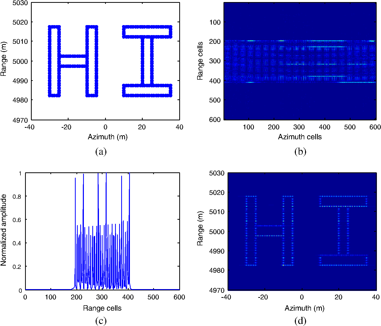

As to the SFW, the conventional range compression method is based on Fourier transform (FT). However, if we directly apply FT to sparse SFWs processing, then the high side-lobes would be generated, just as shown in Figs. 5(a) and 5(b). The proposed range compression method is based on CS theory, which uses the optimizing method instead of FT to complete range compression. Thus, the high side-lobes can be suppressed, just as shown in Figs. 5(c)–5(e). Comparing Fig. 5(d) with Fig. 5(b), we can find that the high-resolution profile is obtained by the proposed method with sparse SFWs. From Fig. 5(e), it can be noted that the imaging result via using the proposed method is clear and close to that with full data, i.e., Fig. 4(d).

Fig. 5

Imaging results of 2-D sparse data: (a) the range profiles by the conventional method; (b) range profile of the 165th pulse; (c) the range profiles by the compressed sensing (CS) method; (d) range profile of the 165th pulse; (e) 2-D imaging result; and (f) Monte Carlo results.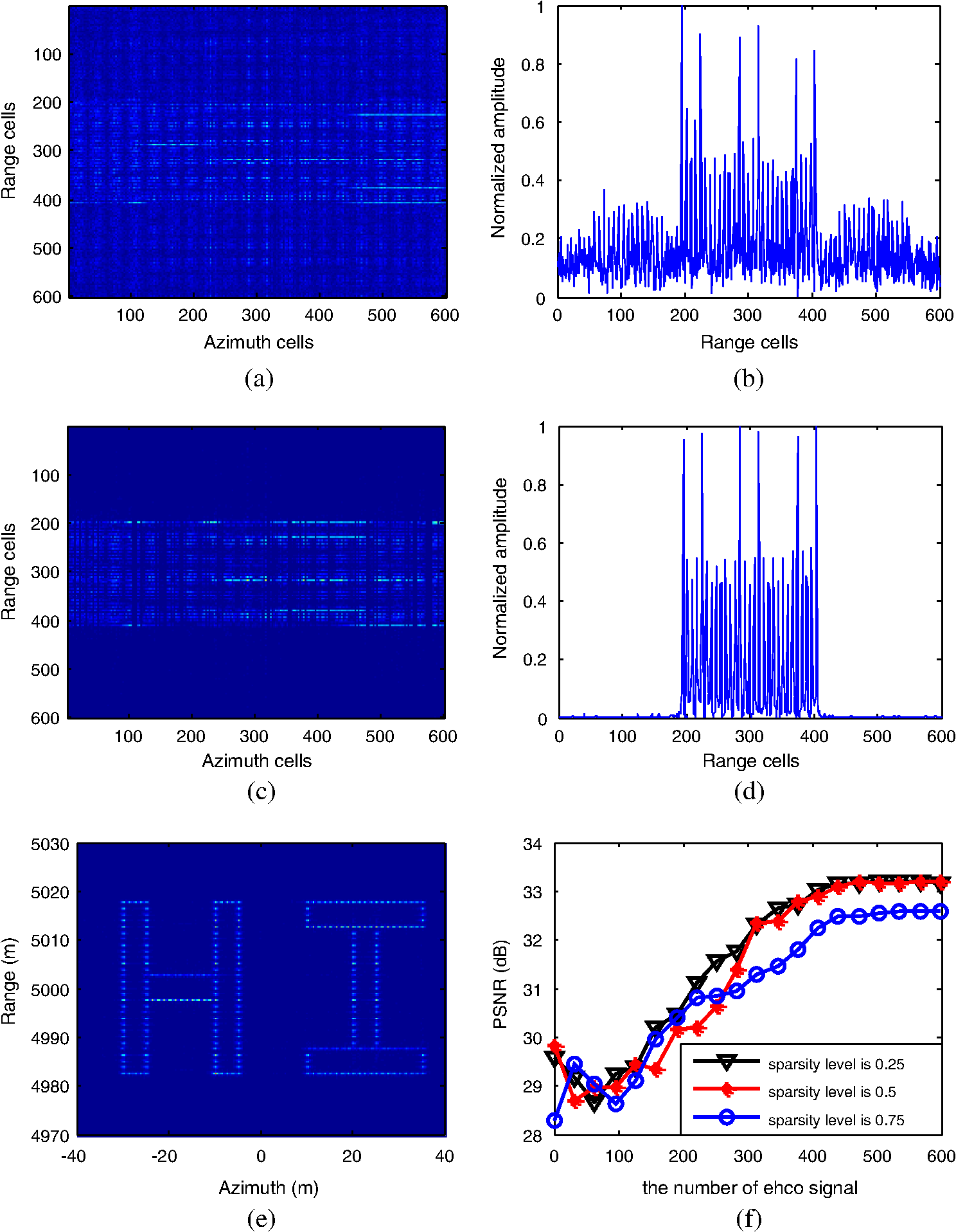

The Monte Carlo method is introduced here to further examine the imaging performance of proposed method with different sparsity levels of transmitted signal and different numbers of echo signals. In the paper, the peak signal-to-noise ratio (PSNR) is utilized to evaluate the quality of the reconstructed images.²¹ The value of PSNR of three different sparsity levels in the frequency domain versus the number of echo signals is shown in Fig. 5(f), where the $x$ -axis denotes the number of echo signals.

From Fig. 5(f), we can find that when the number of echo signals is smaller than 300, the constraint condition cannot be satisfied {the constraint condition is that the dimension of low measurement $M_{1}$ satisfies $M_{1} \geq O (K \log (N_{1}))$ ⁷}. Therefore, the quality of the reconstructed image would be relatively poor and could no longer be accepted. When the number of echo signals is larger than 300, the imaging quality becomes better as the number increases. When the number increases to 450, the PSNR curves saturate, which means that the quality of the imaging result is steady. With a small number of echo signals, the imaging results either of sparsity level 0.25 or of 0.75 are both relatively poor. Thus, the PSNRs are similar. But at a high number, the imaging quality of sparsity level 0.25 is as good as that of sparsity level 0.5; thus the PSNR curves of sparsity level 0.25 and 0.5 are close to each other.

In order to further validate our method, the simulated scene data are utilized in the paper. The imaging parameters are set the same as that of the above simulation. The observed scene is shown as Fig. 6. Figure 7(a) shows the imaging result by using the conventional method with full data. Let the 2-D sparisity levels $(γ, η)$ of the echo data be (0.5, 0.25), (0.5, 0.5), and (0.75, 0.5), respectively. The respective imaging results are shown in Figs. 7(b)–7(d). Visual inspection of these results reveals that the quality of the image is degraded along with the increasing sparsity in accordance with the CS reconstructed theory. However, when the sparisity levels are (0.5, 0.25), the high-quality imaging result is obtained, just as Fig. 8(b). Therefore, the proposed method is valid and feasible.

Fig. 6

Observed scene.

Fig. 7

Image results of area targets with SFW: (a) imaging result with full data; (b) imaging result with sparsity levels (0.5, 0.25); (c) imaging result with sparsity levels (0.5, 0.5); and (d) imaging result with sparsity levels (0.75, 0.5).

Fig. 8

Experiment: (a) experimental scene; and (b) five metal balls in the scene.

5.2.

Performance Analysis with Measured Data

The real data are currently unavailable, so we have to use the experimental data to validate the proposed method. Hence, an experimental platform is set up as shown in Fig. 8(a). The vector network analyzer (VNA) is mounted on a rail to transmit and receive the SFWs. The horn antenna works at a Ka-band. The imaging scene consists of five metal balls, which are shown in Fig. 8(b). During the experiment, the VNA moves on the rail with preset velocity, while the metal balls are fixed. The length of the rail is 1.89 m. The other experimental parameters are shown in Table 1.

Table 1

Synthetic aperture radar (SAR) parameters.

Experimental parameters	Values
Carrier frequency	30 GHz
Frequency-stepped size	3.75 MHz
Number of steps	1600
Bandwidth	6 GHz
Azimuth interval	0.01 m
Number of azimuth cells	189

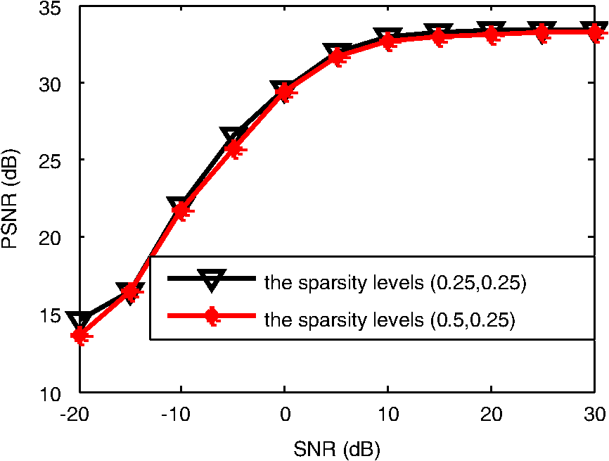
Figures 9(a) and 9(b) show the imaging results obtained by using the conventional method with full data. Figure 9(a) is the range profiles, and Fig. 9(b) is the 2-D imaging result. Figures 9(c) and 9(d) show the imaging results obtained by using the proposed method with the 2-D sparse data, the sparsity level of which is (0.5, 0.25). It can be seen that the proposed CS-based imaging method is effective to get a clear SAR image with the reduced measured data.

Fig. 9

Imaging results of experimental data: (a) range profiles of full data; (b) imaging result of full data; (c) range profiles of 2-D sparse data; and (d) imaging result of 2-D sparse data.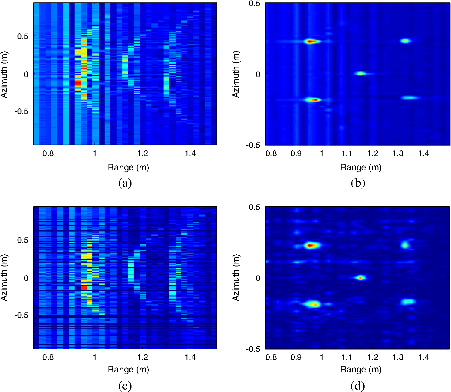

We use the CPU time of recovery as the performance benchmark to evaluate the computational complexity of the proposed and conventional methods. The experiment is run in MATLAB 2007b on a computer with an Intel Pentium 3.1 GHz dual-core processor and 3-GB memory. Regarding the reconstruction time, it requires about 5.2 s to obtain the imaging result by using the proposed method with the sparsity level of (0.5, 0.25), while it requires just about 0.38 s to obtain the conventional imaging result with full data. Although the proposed method needs much more time than the conventional method, the predominance of our method is that a smaller number of frequencies and smaller amount of imaging data are needed for SAR imaging.

In the following, we assume that the received signals are corrupted by uncorrelated additive white Gaussian noise. Let SNR be varied from −20 to 30 dB and the 2-D sparsity levels $(γ, η)$ be (0.25, 0.25) and (0.5, 0.25). We show the value of PSNR versus the SNR in Fig. 10. It can be found that the value of PSNR increases with increasing SNR. However, when the SNR is higher than 10 dB, the value of the PSNR varies very slowly. That is, the quality of the reconstructed image roughly remains steady in this SNR value range.

Fig. 10

Comparison of peak signal-to-noise ratio (PSNR) versus SNR.

6. Conclusion

Conventional SFWs have the disadvantages of poor antijamming capability and requiring a long time period of transmission. Thus, the sparse SFWs are formed, which can improve the antijamming capability and shorten the time period. In the SAR integration time, it frequently occurs that some of the echo data are lost. Thus, a 2-D sparse SAR imaging method is put forward. By using the proposed method, SAR imaging result can be obtained with 2-D sparse data both in the frequency and space domains. In this paper, the proposed method takes advantage of the fact that most natural and manmade signals are compressible. Our future work will include using the uncompressible signals to test the algorithm.

Acknowledgments

This work was supported by the National Natural Science Foundation of China under Nos. 61172169 and 61471386.

References

1.

A. S. KhwajaJ. W. Ma, “Applications of compressed sensing for SAR moving-target velocity estimation and image compression,” IEEE Trans. Instrum. Meas., 60 (8), 2848 –2860 (2011). http://dx.doi.org/10.1109/TIM.2011.2122190 IEIMAO 0018-9456 Google Scholar

2.

Y. Eneset al., “Short-range ground-based synthetic aperture radar imaging: performance comparison between frequency-wavenumber migration and back-projection algorithms,” J. Appl. Remote Sens., 7 (1), 073483 (2013). http://dx.doi.org/10.1117/1.JRS.7.073483 1931-3195 Google Scholar

3.

W. Anet al., “Data compression for multilook polarimetric SAR data,” IEEE Geosci. Remote Sens. Lett., 6 (3), 476 –180 (2009). http://dx.doi.org/10.1109/LGRS.2009.2017498 IGRSBY 1545-598X Google Scholar

4.

B. Hanet al., “A new method for stepped-frequency SAR imaging,” in Proc. of the European Conference on Synthetic Aperture Radar, (2006). Google Scholar

5.

A. Cacciamanoet al., “Contrast-optimization-based range-profile autofocus for polarimetric stepped-frequency radar,” IEEE Trans. Geosci. Remote Sens., 48 (4), 2049 –2056 (2010). http://dx.doi.org/10.1109/TGRS.2009.2035444 IGRSD2 0196-2892 Google Scholar

6.

J. ChenT. ZengT. Long, “A novel high-resolution stepped frequency SAR signal processing method,” in Proc. of IET International Radar Conference, (2009). Google Scholar

7.

D. L. Donoho, “Compressed sensing,” IEEE Trans. Inf. Theory, 52 (4), 1289 –1306 (2006). http://dx.doi.org/10.1109/TIT.2006.871582 IETTAW 0018-9448 Google Scholar

8.

E. CandesJ. RombergT. Tao, “Robust uncertainty principles: exact signal reconstruction from highly incomplete frequency information,” IEEE Trans. Inf. Theory, 52 (2), 489 –509 (2006). http://dx.doi.org/10.1109/TIT.2005.862083 IETTAW 0018-9448 Google Scholar

9.

B. C. ZhangW. HongY. R. Wu, “Sparse microwave imaging: principles and applications,” Sci. China Inf. Sci., 55 (8), 1722 –1754 (2012). http://dx.doi.org/10.1007/s11432-012-4633-4 1674-733X Google Scholar

10.

R. G. BaraniukP. Steeghs, “Compressive radar imaging,” in Proc. of IEEE Radar Conference, 128 –133 (2007). Google Scholar

11.

J. G. Yanget al., “Random-frequency SAR imaging based on compressed sensing,” IEEE Trans. Geosci. Remote Sens., 51 (2), 983 –994 (2013). http://dx.doi.org/10.1109/TGRS.2012.2204891 IGRSD2 0196-2892 Google Scholar

12.

B. Panget al., “Imaging enhancement of stepped frequency radar using the sparse reconstruction technique,” Prog. Electromagn. Res., 140 63 –89 (2013). http://dx.doi.org/10.2528/PIER13030407 PELREX 1043-626X Google Scholar

13.

T. Y. Huanget al., “Cognitive random stepped frequency radar with sparse recovery,” IEEE Trans. Aerosp. Electron. Syst., 50 (2), 858 –870 (2014). http://dx.doi.org/10.1109/TAES.2013.120443 IEARAX 0018-9251 Google Scholar

14.

S. ShahY. YuA. Petropulu, “Step-frequency radar with compressive sampling (SFR-CS),” in Proc. of IEEE International Conference On Acoustics Speech and Signal Processing, (2010). Google Scholar

15.

L. Zhanget al., “High resolution ISAR imaging with sparse stepped-frequency waveforms,” IEEE Trans. Geosci. Remote Sens., 49 (11), 4630 –4651 (2011). http://dx.doi.org/10.1109/TGRS.2011.2151865 IGRSD2 0196-2892 Google Scholar

16.

J.G. Yanget al., “Synthetic aperture radar imaging using stepped frequency waveform,” IEEE Trans. Geosci. Remote Sens., 50 (5), 2026 –2036 (2012). http://dx.doi.org/10.1109/TGRS.2011.2170176 IGRSD2 0196-2892 Google Scholar

17.

H. C. StankwitzM. R. Kosek, “Sparse aperture filled for SAR using super-SVA,” in Proc. of IEEE National Radar Conference, 70 –75 (1996). Google Scholar

18.

R. Baraniuk, “A lecture on compressive sensing,” IEEE Signal Process. Mag., 24 (4), 118 –121 (2007). http://dx.doi.org/10.1109/MSP.2007.4286571 ISPRE6 1053-5888 Google Scholar

19.

G. H. MohimaniM. Babaie-ZadehC. Jutten, “A fast approach for overcomplete sparse decomposition based on smoothed norm,” IEEE Trans. Signal Process., 57 (1), 289 –301 (2009). http://dx.doi.org/10.1109/TSP.2008.2007606 ITPRED 1053-587X Google Scholar

20.

E. CandesT. Tao, “Near optimal signal recovery from random projections: universal encoding strategies?,” IEEE Trans. Inf. Theory, 52 (12), 5406 –5425 (2006). http://dx.doi.org/10.1109/TIT.2006.885507 IETTAW 0018-9448 Google Scholar

21.

S. Y. YangD. L. PengM. Wang, “SAR image compression based on bandelet network,” in Proc. of IEEE Fourth International Conference on Natural Computation, 559 –563 (2008). Google Scholar

Biography

Fufei Gu received his MS degree in electrical engineering from the Institute of Information and Navigation, Air Force Engineering University (AFEU), Xi’an, China, in 2011, where he is currently working toward his PhD degree in electrical engineering. He is currently with the Radar and Signal Processing Laboratory, Institute of Information and Navigation, AFEU. His research interests include compressed sensing theory and radar imaging.

Qun Zhang (M’02–SM’07) received his MS degree in mathematics from Shaanxi Normal University, Xi’an, China, in 1988, and the PhD degree in electrical engineering from Xidian University, Xi’an, in 2001. He is a senior member of the Chinese Institute of Electronics (CIE), a committee member of the Radiolocation Techniques Branch, CIE. He is currently a professor with the Institute of Information and Navigation, Air Force Engineering University, Xi’an, and an adjunct professor with the Key Laboratory of Wave Scattering and Remote Sensing Information (Ministry of Education), Fudan University, Shanghai, China.

Hao Lou received his MS degree in electrical engineering from the Institute of Electronic and Electric, National University of Defense University, Changsha, China, in 2008. Since 2012, he had been working toward his PhD degree in electrical engineering in the Institute of Information and Navigation, Air Force Engineering University. His research interests include radar-communication integration and radar signal processing

Zhi’an Li received his MS degree from Naval Engineering University, Wuhan, China, in 2003. He is currently a professor with the Institute of Information and Navigation, Air Force Engineering University, Xi’an. His research interests include airborne radar and navigation.

Ying Luo received his MS degree in electrical engineering from the Institute of Telecommunication Engineering, Air Force Engineering University (AFEU), Xi’an, China, in 2008, and the PhD degree in electrical engineering from AFEU, in 2013. He is currently working in the Key Laboratory for Radar Signal Processing, Xidian University, as a postdoctoral fellow. His research interests include signal processing and ATR in SAR and ISAR.

CC BY: © The Authors. Published by SPIE under a Creative Commons Attribution 4.0 Unported License. Distribution or reproduction of this work in whole or in part requires full attribution of the original publication, including its DOI.

Citation Download Citation

Fufei Gu, Qun Zhang, Hao Lou, Zhi’an Li, and Ying Luo "Two-dimensional sparse synthetic aperture radar imaging method with stepped-frequency waveform," Journal of Applied Remote Sensing 9(1), 096099 (7 January 2015). https://doi.org/10.1117/1.JRS.9.096099

Published: 7 January 2015

Access the abstract

JOURNAL ARTICLE
16 PAGES

DOWNLOAD PAPER SAVE TO MY LIBRARY