|
|
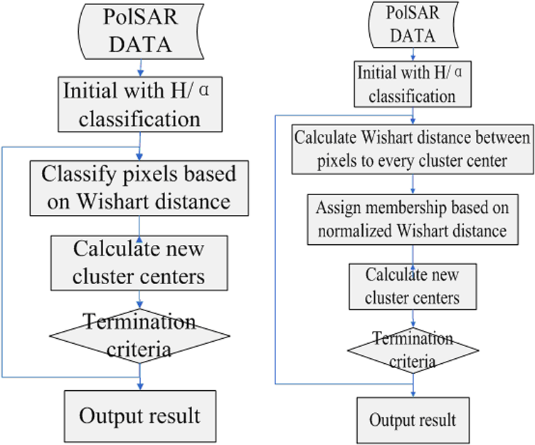
1.IntroductionLand cover classification is one of the major applications of polarimetric synthetic aperture radar (PolSAR).1 The PolSAR system can work continuously in all weather and can take advantage of four kinds of polarization to obtain a wealth of feature information about features, which has broad application prospects.2 However, PolSAR images are seriously influenced by speckle noise, which leads to major difficulties in image classification.3 Over the last two decades, researchers have proposed many classification methods for PolSAR images.4,5 In 1989, Van Zyl suggested that the PolSAR data could be classified into four kinds of scattering mechanisms, namely, even number of reflections, odd number of reflections and diffuse scattering, volume, and nonseparable scattering.6 Then Freeman and Durden developed a new model to describe the polarimetric signature including volume, and the Bragg scattering mechanisms,7 whose experimental results showed that the approach could deliver clear discrimination between different types of scene pixels. In 1995, scattering entropy, introduced by Cloude,8 was first used in SAR image classification and later Cloude–Pottier proposed a classification algorithm based on the decomposition.9 However, a deficiency of the algorithm is that it cannot effectively distinguish different topographic features whose pixels are in the same area. Subsequently, a method combined the decomposition with an iterative Wishart clustering algorithm, and was proposed by Lee et al. in 1999.10 Among these, the -Wishart method proposed by Lee has been widely used because it has a more stable performance than other algorithms.11 However, because the algorithm uses the hard C-means framework, the clusters are divided in an arbitrary way, which makes the algorithm too sensitive to noise. Because the classification results still have difficulty in meeting application requirements, there is still room for improvement in classification accuracy. The fuzzy set concept can solve the problem with traditional set theory, which performs a rigid division of set elements.12 In fuzzy set theory, an element can belong to several sets at the same time, with a certain degree of membership in each one. The introduction of fuzzy partitions can overcome the shortcoming that the algorithm results are too sensitive to isolated points.13 A PolSAR image consists of the scattering echo of various surface features in the observation area,14 and an image pixel often contains a variety of basic scattering types, which means that simply classifying a pixel as a certain type is not reasonable. At the same time, this is the main reason why the fuzzy set concept is a convenient classification method for PolSAR images. Currently, many remote-sensing image classification methods make use of fuzzy set theory. Mao introduced fuzzy set theory to cerebellar model arithmetic computer (CMAC) neural networks and proposed a method that reflects the fuzziness of human cognition and the continuity of fuzzy CMAC neural networks.15 The results show that the classification accuracy of this approach is significantly higher than that of the traditional maximum likelihood classification method. Liu et al. used semisupervised learning theory and the core theory of the fuzzy C-means (FCM) algorithm to improve classification accuracy.16 Obviously, fuzzy theory can be applied to improve the accuracy of classification results in two main ways: directly used to improve existing methods or combined fuzzy theory or the FCM algorithm with a novel algorithm.17 In recent years, some researchers have applied fuzzy theory to image classification and achieved good results for PolSAR images.18–20 However, these methods directly use the FCM algorithm, which does not associate polarization parameters with fuzzy sets. Therefore, in this paper, the fuzzy concept is added to the -Wishart algorithm to enable fuzzy clustering based on the Wishart distance to obtain more reasonable classification results. To verify the effectiveness of the proposed algorithm, three sets of PolSAR image data are experimentally analyzed. The rest of the paper is organized as follows. Necessary background information and fundamental knowledge are provided in Sec. 2. Details of the proposed unsupervised classification algorithm are described in Sec. 3. Section 4 describes the remote-sensing datasets used, together with experimental results and discussion. The conclusions are presented in Sec. 5. 2.Background2.1.PolSAR DataThe basic form of PolSAR data is the Sinclair scattering matrix using horizontal and vertical matrices, expressed by Eq. (1): where is the scattering matrix element of horizontal-vertical polarization. For the complex Pauli spin matrix set, the matrix can be transformed to the three-dimensional Pauli vector, as Eq. (2):Then the coherency matrix can be obtained as shown in Eq. (3): where , , and . The superscript denotes transpose, and “*” is the complex conjugate.2.2.Fuzzy Set TheoryFuzzy set theory emerged in the nineteenth century and transformed classic two-valued logic into a continuous logic in the closed interval [0, 1], which was more in line with the human brain’s cognitive and reasoning processes. The main difference between traditional set theory and fuzzy set theory is the mechanism of element membership. In traditional set theory, there are only two kinds of collection mechanisms {Yes or No}, for which a quantitative description is ; that is, an element can either belong to or not belong to a set. In fuzzy set theory, the concept of membership is introduced, and an element can be assigned a grade of membership from 0 to 1. This expansion means that an element can belong to multiple collections at the same time, with different degrees of membership in each. Compared to traditional set theory, fuzzy sets smooth the process of translation between quantitative and qualitative representations. 2.3.Classifier Based on Target DecompositionIn 1996, Cloude and Pottier proposed a target decomposition method based on a coherency matrix.21 The coherency matrix is first decomposed into the sum of the products of eigenvalues and eigenvectors, as shown in Eq. (4): where are the eigenvalues and are the eigenvectors, and denotes transpose. Then the entropy and scattering angle can be decomposed as in Eq. (5):H and can be used to define a two-dimensional feature space. Cloude and Pottier proposed the classification boundaries of the plane on the basis of a large number of experiments.9 Using this approach, the PolSAR data can be divided into eight classes based on Fig. 1. 2.4.-Wishart AlgorithmAccording to Goodman,22 the coherency matrix obeys the complex Wishart distribution, and its probability density is as shown in Eq. (6): where is the expectation of the coherency matrix , is the number of images, is a normalization coefficient, Tr represents the trace of the matrix, and is the gamma function. represents the monostatic backscattering case, while represents the bistatic case.Lee et al. proposed the -Wishart algorithm based on the maximum likelihood decision criterion.10 The Wishart distance between the coherency matrix of the pixel and the cluster center of the target class can be expressed as in Eq. (7): where is the mean of the coherency matrix of all the pixels belonging to class . In the -Wishart algorithm, when the coherency matrix of a pixel satisfies Eq. (8), the pixel will be classified into class . Because the category of an element depends only on the minimum distance between this element and the center of every class, the -Wishart algorithm uses the rigid C-means algorithm. This means that eight initial classes are obtained based on the two parameters H and , and then iterative clustering is performed using the Wishart distance by means of the classification process shown in Fig. 2(a). As shown in the figure, the new cluster center is calculated by taking the average of the matrix of all pixels belonging to the corresponding class. The calculation method is shown in Eq. (9): where is the total number of pixels, is the cluster center of class , and represents the coherency matrix for pixel . When the ’th pixel belongs to class , takes on a value of 1; otherwise, it is 0. The end condition is that the number of pixels that change category between two generations is less than a given threshold value or that the number of iterations reaches a given threshold value.2.5.Fuzzy Clustering Based on Wishart DistanceTo solve the problem of inflexible clustering, an -Wishart fuzzy clustering algorithm based on the Wishart distance is proposed in this paper, which allows pixels to belong to more than one class with a certain degree of membership for each. According to the concept of fuzzy set theory, the degree of membership of one point in a given class shall be 1 when the distance from this point to the class center is small enough, meaning that the point completely falls into this class and that the degree of membership of this point in other classes must be 0. When no class satisfies this condition, the degree of membership of a given point shall be set according to the distance between that point and the center of every class; the further away the point, the less will be the degree of membership. In addition, when a point completely belongs to a certain class, the sum of its memberships in every class is 1, and this condition shall still be satisfied when the point belongs to several classes. After introducing the concept of membership, the method of computing the class center is still Eq. (6), but the meaning of has been expanded to be the degree of the membership of pixel in class , and its value range has changed from to the interval [0,1]. The improved classification process is shown in Fig. 2(b). 3.-Fuzzy Wishart ClassifierBased on the concept described above, the - fuzzy Wishart classifier was designed in this paper. The concrete implementation of the process was as described below. 3.1.Image PreprocessingDue to imaging system complexity and real-world imaging factors, PolSAR images usually contain much noise, but its influence can be reduced by filtering operations. In this research, a refined Lee filter with a window was applied before the classification experiments. 3.2.InitializationIn this initial step, images are classified into eight categories to initialize the cluster centers with classifier. The initial process is as follows:
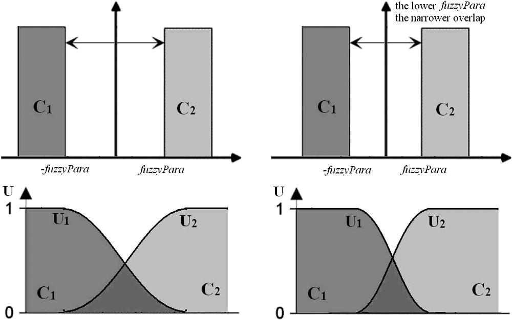
3.3.Fuzzification of Wishart Distance State SpaceBased on the cluster centers calculated in Sec. 3.2, one of the key points in this paper, the design of the fuzzy membership functions (FMFs), can be done. In order to fuzzify the Wishart distance state space, let represent the degree of the fuzzy membership with which the ’th point belongs to the ’th class. The FMFs satisfy the following conditions over the entire state space: where is the total number of clusters. For the ’th pixel, Wishart distances between clusters can be computed according to Eq. (7), and let represent the Wishart distance between the ’th pixel and ’th cluster.Because of terrain, sensor type, the wavelength of the electromagnetic waves used for measurement, and various other reasons, the values of the Wishart distance vary over a wide range. In fact, because the calculation of the Wishart distance involves a logarithmic operation, as can be seen in Eq, (7), the Wishart distance can even be negative. All these reasons prevent regular membership calculation and fuzzy partition. Therefore, to make the membership calculation feasible and to solve the problem of setting an appropriate unified threshold for the fuzzy partition of an arbitrary domain, a normalization of Wishart distance for every pixel is performed as shown in Eq. (12): where a sample group is the Wishart distances from ’th point to each cluster, is the total number of clusters, is the normalized distance, is the variance of the sample group, and is the average of the Wishart distances from ’th point to every cluster, namely the sample mean. Then the fuzzy membership can be specified as follows:For ’th point, there can be two different conditions: totally belonging to one cluster or belonging to several clusters at same time. When the normalized distance between this point and the ’th cluster center is small enough, this point shall totally belong to the ’th class as shown by Eqs. (13) and (14): where represents the degree of the fuzzy membership with which the ’th point belongs to the ’th class and is a parameter introduced in the fuzzy function design to adjust the range of acceptance of fuzzy operation. Otherwise, when the distances between ’th point and every cluster center are all larger than , the point shall belong to several clusters and a judgment shall be made to choose the essential clusters as shown by Eqs. (15) and (16): where means the minimum value of and , which can ensure the pixel far from the cluster center has no effect on the membership calculation. And means the distance between ’th point and ’th cluster is too large so that the membership of ’th point to ’th cluster shall be set to 0.3.4.Update of Cluster Center and Iterative Refinement of ClusteringAfter the fuzzy membership degrees have been determined in Sec. 3.3, the new cluster center can be computed based on Eq. (17): where is the total number of pixels, is the new cluster center of class , and represents the coherency matrix for pixel . Comparing Eq. (17) with Eq. (9), the major improvement of the fuzzy clustering algorithm is that the weighting parameter in Eq. (9) must be 0 or 1, while in Eq. (17) can have value from 0 to 1.With the cluster centers updated, the categories of every pixel can be reclassified based on Eqs. (7) and (8). And then an iteration of Secs. 3.3 and 3.4 can be done until the terminating condition is met. 3.5.Stopping ConditionThe stopping condition is different in different applications. One option is to set a fixed number of iteration times, and another option is to set a fixed threshold of the number of pixels that change categories between two consecutive iterations. When the maximum iteration number is met, or the change rate is less than the threshold, output the classification result. Otherwise, return to Sec. 3.3. Finally, the proposed algorithm outputs a classification image. 3.6.Parameter AdjustmentBecause of variations in the data distribution, the parameter is introduced in the fuzzy function design to adjust the range of acceptance of fuzzy operation. When the data separate well and are easy to cluster, a small can be used. When the data have a disorderly distribution and are difficult to classify, a larger can be used to expand the range of acceptance of fuzzy operation to improve algorithm performance. Figure 3 shows how the parameter affects the fuzzification of two categories as a simple case. 4.Application and DiscussionTo verify the effectiveness of the proposed method, experiments were done using three datasets. The first consists of full-polarimetric SAR data for San Francisco Bay, California, obtained from NASA-JPL AIRSAR in 1992. The size of the experimental dataset is . The region includes urban areas, ocean, vegetation, the Golden Gate Bridge, and other targets. The second consists of L-band PolSAR data for the Flevoland region from the NASA/JPL Laboratory AIRSAR sensor in 1989, with an azimuth resolution of 12.10 m and a distance resolution of 6.6 m. The feature types in the experimental area are relatively simple; most are croplands of rectangular shape, including grassland, potatoes, alfalfa, wheat, soybeans, sugar beets, peas, and other target surface features. The size of the experimental dataset is . And the third consists of X-band full-polarimetric high-resolution SAR data for LingShui town in Hainan Province, China, in 2010. The original size of this dataset was . The region includes airport runways, urban areas, pools, and various kinds of croplands, such as red peppers, betel palms, mangoes, papayas, and rice paddies. Because the original dataset was too large for analysis, a subarea sized was selected for the experiments. Results were compared between the proposed method and the -Wishart algorithm. 4.1.Experiment 1: L-Band PolSAR Image of San Francisco BayThe first dataset and the classification results are shown in Fig. 4. Several basic features, such as ocean, beach, mountains, vegetation, urban areas, and noise, in the upper-right corner can be clearly seen in Fig. 4(a). The water has low-entropy surface scattering, the bare soil has medium-entropy surface scattering, the vegetation has medium-entropy vegetation scattering, and the urban areas have high-entropy volume scattering. These major ground features in San Francisco Bay are more distinguishable. Experiment 1 is done to check the performance of the proposed algorithm in classifying the ground features with different kinds of scattering types. Fig. 4San Francisco data and classification results. (a) PauliRGB image. (b) -Wishart result. (c) -Wishart fuzzy clustering result. 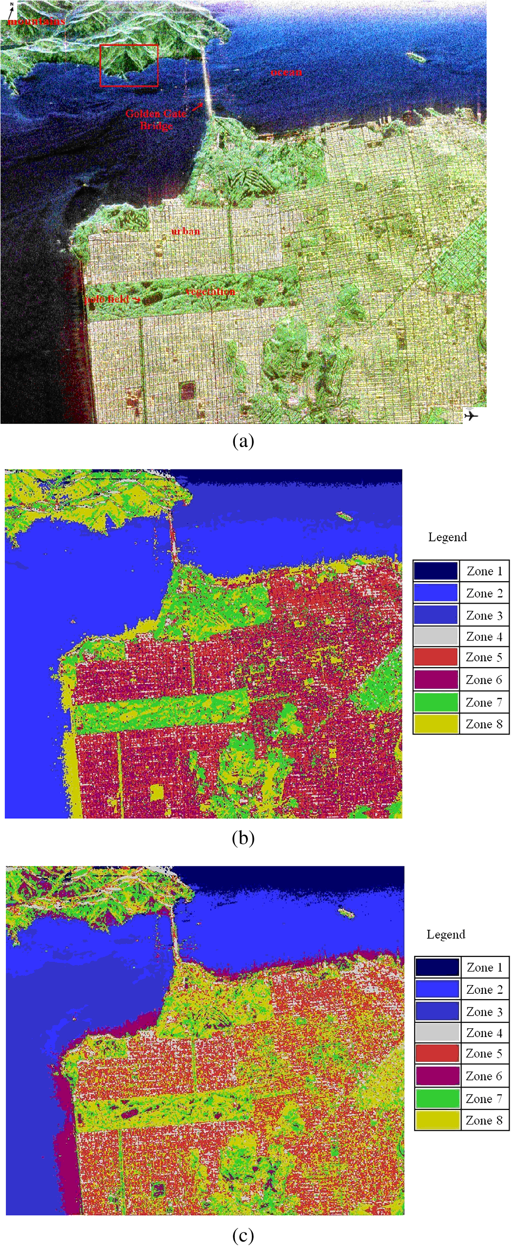 According to the types indicated in Fig. 4(a), in the classification results of the -Wishart algorithm shown in Fig. 4(b), the first zone corresponds to noise. The corresponding feature type of the second and third zones is ocean. The fourth, fifth, and sixth zones correspond to urban areas. The seventh zone corresponds to vegetation and the eighth to bare land. The algorithm effectively distinguishes several basic features of the marine, urban, vegetation, and bare land environments, but some yellow spots representing bare land are evident in the blue zone representing the ocean, which is obviously a misclassification. Moreover, the urban areas are divided into three classes, which seem to be unreasonable and overly complex because each of the separate zones has no distinguishing characteristic. Figure 4(c) shows the classification results for -Wishart fuzzy clustering. Similar to the types indicated in Fig. 4(a), the first zone corresponds to noise, and the second and third zones correspond to ocean. The fourth and fifth zones correspond to urban areas. The sixth, seventh, and eighth zones all correspond to bare land. Comparing Fig. 4(c) with Fig. 4(b), it can be seen that in the classification results of the -Wishart fuzzy clustering method, the misclassified spots, which were classified as ocean, are now correct, and urban areas and vegetation are reasonably divided into two classes. Furthermore, there is a large difference between the classification results of -Wishart and of the -Wishart fuzzy clustering algorithm in the oval shown in Fig. 5. Fig. 5Detailed comparison of San Francisco data classification results. (a) PauliRGB image. (b) -Wishart result. (c) -Wishart fuzzy clustering result.  In the area in the upper left of Fig. 4(a) marked by a red box, at the back of a mountain, there is a shadow area in the image because the higher terrain blocks the other parts of the back slope, which leads to less effective reception of information. The shaded area is similar to a calm water surface in its polarization characteristics, therefore, in the -Wishart classification result, this section is almost completely classified as ocean. However, in the -Wishart fuzzy clustering result, the algorithm is able to find a more reasonable cluster center, which leads to most of those pixels being classified more reasonably as bare land. Experimental results show that the classification accuracy of the improved algorithm proposed in this paper is greatly increased over that of the -Wishart method. To validate the improvements in fuzzy clustering achieved by calculating cluster centers, the movement paths of the cluster centers have been tracked. Figures 6(a) and 6(b) show the movement paths of the cluster centers as calculated by the -Wishart and the -Wishart fuzzy clustering algorithm. The background is the data distribution in the plane, the transition from red to dark blue represents the density change from high to low, and the hollow points indicate the final positions of the cluster centers. The combination of the cluster center locations and the data distribution in the plane reflects the effectiveness and reasonableness of the cluster centers. Figure 6(a) shows that there were five cluster centers that were calculated by the H/a-Wishart algorithm and located in the medium-entropy multiple-scattering region, with the first and fifth cluster centers slightly distant from the data-intensive region. In Fig. 6(b), the cluster centers calculated by the proposed method eventually moved to the data-intensive region and distributed themselves evenly. The classification results indicate that the clustering density of the proposed method is more reasonable, while the clustering density of the -Wishart algorithm is uneven because the urban areas were divided into three classes and the gray part contained only a few pixels, which seemed to be insignificant. 4.2.Experiment 2: L-Band PolSAR Image of FlevolandTo further verify the validity of the classification algorithm, the second set of PolSAR data was used for another set of experiments and a quantitative analysis was performed using a confusion matrix. Most feature types in this experimental area are croplands, including grassland, potatoes, alfalfa, wheat, soybeans, sugar beets, peas, and other target ground features, which usually result in medium-entropy vegetation scattering. Experiment 2 is done to check the performance of the proposed algorithm in classifying the different ground features with similar kinds of scattering types. Figure 7(a) shows an RGB composite image of the region. The red, green, and blue components of the composite image were obtained using the three parameters , , and derived from the Pauli decomposition. Fig. 7Flevoland data Pauli image and classification results. (a) Pauli composite image of the Flevoland experimental zone. (b) -Wishart classification result. (c) -Wishart fuzzy clustering result. 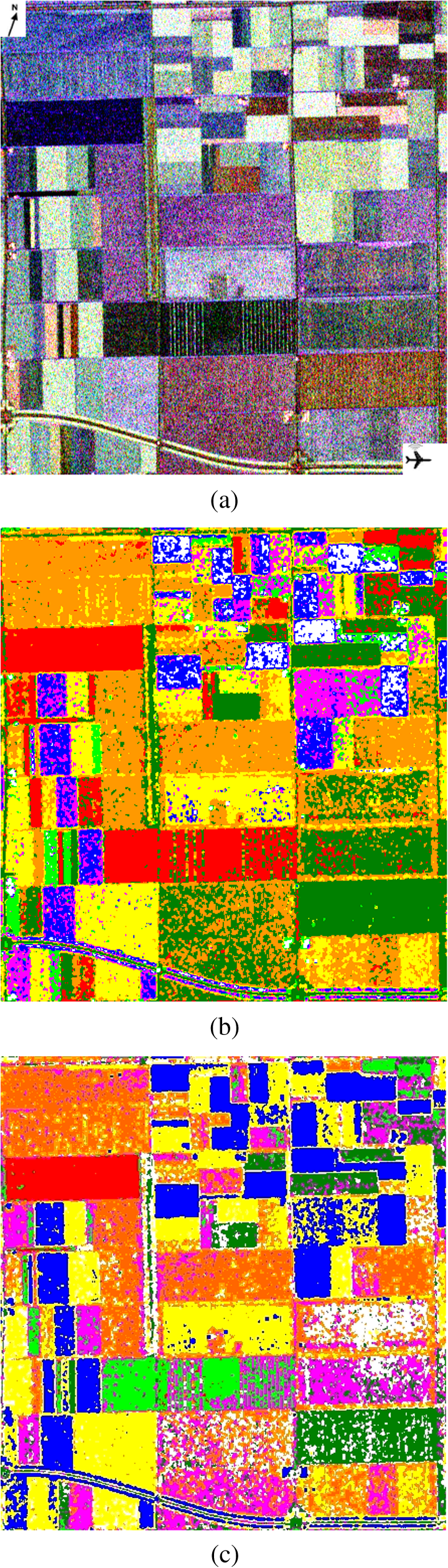 Comparing Figs. 7(b) and 7(c), the classification result from the fuzzy clustering method is much smoother than from the other method. In the results of the -Wishart algorithm, some areas were not distinguished, such as peas, while some other types were misclassified into several classes, such as lawns and potatoes. However, the majority of surface features, such as peas and beets, can be identified correctly in the -Wishart fuzzy clustering result. The stretch of road at the bottom of this area and the edges of every field in the fuzzy clustering results are both clearer than the -Wishart algorithm. To evaluate the classification accuracy, Fig. 8 shows the reference image of the real surface features, and the six major class samples from the image that were selected to compute the confusion matrices. As can be seen from Table 1, the accuracy of the -Wishart fuzzy clustering algorithm is greater than that of the -Wishart method, both in terms of overall accuracy and Kappa coefficient. For some categories, such as rape, bare land, and lawn, the mapping accuracy and precision of the two methods are both . For most classes, the accuracy of the -Wishart fuzzy clustering algorithm is always a little better because the misclassified points in each zone are fewer with the fuzzy operation. Table 1Confusion matrices of H/α-Wishart and fuzzy clustering algorithm.
4.3.Experiment 3: X-Band High-Resolution PolSAR Image of LingShui, HainanThe third dataset was collected from the farmland surrounding LingShui. Fields and roads can be easily distinguished in Fig. 9(a), where the green lines mark areas where crops grow lushly and almost completely cover the land, appearing as massive objects, the blue lines mark areas where the plants are small and the soil is bare, as reflected in the strip shapes in the image, and the black blocks are pools. Experiment 3 is done to check the performance of the proposed algorithm in classifying the high-resolution ground features. Fig. 9LingShui, Hainan, data and classification results. (a) PauliRGB image. (b) -Wishart result. (c) -Wishart fuzzy clustering result.  Figure 9(b) shows that the -Wishart method was less effective in generating accurate clusters. In the vegetation zone, categories are mixed, creating many small spots. As many as six categories can be seen in a small region. There was obvious misclassification in the region indicated by black circles, where parts of roads, which generate a low-intensity response, were mistakenly classified as water. The -Wishart fuzzy clustering algorithm improved the classification results and yielded a clearer clustering in which few of the pixels representing roads were classified as water. Figure 10 clearly shows that, compared with the -Wishart method, the improved algorithm did a better job of distinguishing shadows from water. Fig. 10Detailed comparison of LingShui, Hainan, data classification results. (a) PauliRGB image. (b) -Wishart result. (c) -Wishart fuzzy clustering result.  The region shown in Fig. 10(a) bounded by red lines [as shown in Fig. 9(a) in the corresponding red rectangle] is a grove of mangoes. The synthetic map shows that the presence of trees above the ground created shadows as shown in Fig. 10(a), where the intensity of the echo is weak in the bottom-right portion of the mango trees, which are colored in black. In the results of the -Wishart method, most of the shadows were mistakenly classified as water, while in the results of the -Wishart fuzzy clustering algorithm, due to the fuzzy concept, the cluster centers moved to a more reasonable position, causing the pixels in that region to be reclassified, with only a small group remaining misclassified. To further evaluate the performance of the new algorithm, the classification results for five typical kinds of land cover according to Fig. 11 are summarized in Table 2. In the results of the -Wishart algorithm, grassy plant and woody plant classes are both classified into several classes, which seem rather messy and result in low accuracy; most of the bare soil is classified as plants or paths, while only 35.88% are in the correct category. In the results of the -Wishart fuzzy clustering algorithm, of the grassy plant and woody plant pixels are in correct categories, which proves that fuzzy logic can lead to a softer clustering and can classify a small group of isolated pixels into a larger class. While the accuracy of the path class is lower than the -Wishart result, this seems to be the price for improving the classification accuracy of water and shadow because the algorithm used more categories to differentiate water, bare soil, paths in fields, and shadows. Fig. 11Locations of test samples: grassy plants (green circle), woody plants (red square), bare soil (orange triangle), paths (blue diamond), water (red upside down triangle). 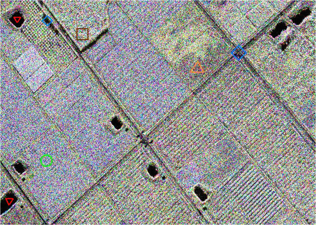 Table 2Confusion matrices of H/α-Wishart and fuzzy clustering algorithm for LingShui data.
By integrating the results of these three sets of experiments, the improved algorithm proposed in this paper can effectively improve classification accuracy and achieve a reasonable classification of shadows and water. 5.ConclusionsTo solve the problem of inflexible clustering in the hard C-means clustering model used by the -Wishart algorithm, fuzzy concepts, which can blur pixel class boundaries, have been introduced into the proposed -Wishart fuzzy clustering algorithm. Three kinds of real-world PolSAR images were used in the classification experiments. Results show that the fuzzy clustering algorithm based on fuzzy set theory performed better in terms of classification accuracy than the -Wishart algorithm and can effectively solve the problem of misclassifying shadows and water. In the algorithm proposed in this paper, further research remains to be done on the automatic setting of the fuzzy parameter and the exact distribution of normalized data. At the same time, it would also be worthwhile to explore why improving the positions of the cluster centers by fuzzy clustering can correct the misclassification of shadows and water. AcknowledgmentsThis study is supported by three Chinese foundations: the National High Technology Research and Development Program of China (Grant No. 2011AA120404), Scientific Research Base Development Program of the Beijing Municipal Commission of Education, and Research on Object Oriented Refined Classification Method of High Resolution Woodland Synthetic Aperture Radar Image (No. 201320). ReferencesH. K. YuY. H. ZhangY. J. Wang,
“The research of land cover classification using polarimetric SAR data,”
Hydrogr. Surv. Charting, 26
(3), 34
–38
(2006). Google Scholar
C. Xieet al.,
“Multitemporal polarimetric SAR data fusion for land cover mapping,”
Remote Sens. Land Resour., 22
(3), 120
–124
(2010). http://dx.doi.org/10.1109/GEOINFORMATICS.2010.5567565 Google Scholar
Z. S. Zhanget al.,
“Research on polarimetric SAR image speckle reduction using kernel independent component analysis,”
Acta Geodaetica et Cartographica Sinica, 40
(3), 290
–295
(2011). Google Scholar
L. Ferro-FamilE. PottierJ. S. Lee,
“Unsupervised classification of multifrequency and fully polarimetric SAR images based on the H/A/alpha-Wishart classifier,”
IEEE Trans. Geosci. Remote Sens., 39
(11), 2332
–2342
(2001). http://dx.doi.org/10.1109/36.964969 IGRSD2 0196-2892 Google Scholar
R. GuoX. R. BaiM. D. Xing,
“Unsupervised classification of fully polarimetric SAR image based on deorientation theory,”
Mod. Radar, 32
(4), 35
–38
(2010). Google Scholar
J. Van Zyl,
“Unsupervised classification of scattering behavior using radar polarimetry data,”
IEEE Trans. Geosci. Remote Sens., 27
(1), 36
–45
(1989). http://dx.doi.org/10.1109/36.20273 IGRSD2 0196-2892 Google Scholar
A. FreemanS. L. Durden,
“A three-component scattering model for polarimetric SAR data,”
IEEE Trans. Geosci. Remote Sens., 36
(3), 963
–973
(1998). http://dx.doi.org/10.1109/36.673687 IGRSD2 0196-2892 Google Scholar
S. R. Cloude,
“An entropy based classification scheme for polarimetric SAR data,”
in Int. Geoscience and Remote Sensing Symp.,
2000
–2002
(1995). Google Scholar
S. R. CloudeE. Pottier,
“An entropy based classification scheme for land applications of polarimetric SAR,”
IEEE Trans. Geosci. Remote Sens., 35
(1), 68
–78
(1997). http://dx.doi.org/10.1109/36.551935 IGRSD2 0196-2892 Google Scholar
J. S. Leeet al.,
“Unsupervised classification using polarimetric decomposition and the complex Wishart classifier,”
IEEE Trans. Geosci. Remote Sens., 37
(5), 2249
–2258
(1999). http://dx.doi.org/10.1109/36.789621 IGRSD2 0196-2892 Google Scholar
J. S. Leeet al.,
“Unsupervised terrain classification preserving polarimetric scattering characteristics,”
IEEE Trans. Geosci. Remote Sens., 42
(4), 722
–731
(2004). http://dx.doi.org/10.1109/TGRS.2003.819883 IGRSD2 0196-2892 Google Scholar
J. YangF. K. LangD. R. Li,
“An unsupervised Wishart classification for fully polarimetric SAR image based on Cloude-Pottier decomposition and polarimetric whitening filter,”
Geomatics Inf. Sci. Wuhan Univ., 36
(1), 104
–107
(2011). Google Scholar
L. YangW. LiuZ. G. Wang,
“Weighted-based unsupervised Wishart classification of fully polarimetric SAR image,”
J. Electron. Inf. Technol., 3
(12), 2827
–2830
(2008). http://dx.doi.org/10.3724/SP.J.1146.2007.00950 Google Scholar
W. L. WuY. M. PiQ. He,
“Classification of fully polarimetric SAR image using AdaBoost algorithm,”
Signal Process., 25
(10), 1594
–1597
(2009). SPRODR 0165-1684 Google Scholar
J. X. MaoY. N. WangW. Sun,
“Remote sensing image classification algorithm based on fuzzy CMAC neural network,”
Acta Geodaetica et Cartographica Sinica, 31
(4), 327
–332
(2002). Google Scholar
X. F. LiuB. B. HeX. W. Li,
“Classification for Beijing-1 micro-satellite’s multispectral image based on semi-supervised kernel FCM algorithm,”
Acta Geodaetica et Cartographica Sinica, 40
(3), 301
–306
(2011). Google Scholar
A. Reigberet al.,
“Polarimetric fuzzy K-means classification with consideration of spatial context,”
(2014) http://earth.esa.int/workshops/polinsar2007/presentations/154_reigber.pdf December ). 2014). Google Scholar
P. R. KerstenJ. S. LeeT. L. Ainsworth,
“Unsupervised classification of polarimetric synthetic aperture radar images using fuzzy clustering and EM clustering,”
IEEE Trans. Geosci. Remote Sens., 43
(3), 519
–527
(2005). http://dx.doi.org/10.1109/TGRS.2004.842108 IGRSD2 0196-2892 Google Scholar
J. Yuet al.,
“Unsupervised classification for polarimetric synthetic aperture radar image using the fuzzy possibilistic C-means clustering,”
in 2010 2nd Conf. on Environmental Science and Information Application Technology,
72
–75
(2010). Google Scholar
T. ZhangJ. T. SunR. L. Yang,
“Fuzzy classification of polarimetric SAR images,”
Syst. Eng. Electron., 33
(5), 1036
–1040
(2011). Google Scholar
S. R. CloudeE. Pottier,
“A review of target decomposition theorems in radar polarimetry,”
IEEE Trans. Geosci. Remote Sens., 34 498
–518
(1996). http://dx.doi.org/10.1109/36.485127 IGRSD2 0196-2892 Google Scholar
N. R. Goodman,
“Statistical analysis based on a certain multivariate complex Gaussian distribution,”
Ann. Math. Stat., 34 152
–177
(1963). http://dx.doi.org/10.1214/aoms/1177704250 AASTAD 0003-4851 Google Scholar
BiographyTeng Zhu received his BS degree in soft engineering from Wuhan University, China, in 2010. Now, he is studying remote-sensing image processing, artificial intelligence, and pattern recognition for the PhD in the School of Remote Sensing and Information Engineering, Wuhan University, China. Yu Jie received her doctor degree in Wuhan University from 1996.09 to 2002.12. She is currently professor of GIS and remote sensing at Wuhan University. She has been involved in a number of projects funded by the State Bureau of Surveying and Mapping. She won the provincial science and technology progress second prize twice, Hubei Province Natural Science outstanding paper award, and the outstanding youth teacher award three times. Li Xiaojuan is a professor in the College of Resource Environment and Tourism and the Beijing Key Laboratory of Resource Environment and Geographic Information System at Capital Normal University. She is engaged in teaching and research about resource and environment information systems and environmental remote sensing Jie Yang received the PhD degree from Wuhan University, Wuhan, China, in 2004. Since 2011, he has been a professor with the State Key Laboratory of Information Engineering in Surveying, Mapping, and Remote Sensing, Wuhan University. His main current research interests are in understanding synthetic aperture radar images. |