Economic impacts of climate change on agriculture: the AgMIP approach

Jacques Delincé; Pavel Ciaian; Heinz-Peter Witzke

doi:10.1117/1.JRS.9.097099

21 January 2015 Economic impacts of climate change on agriculture: the AgMIP approach

Jacques Delincé, Pavel Ciaian, Heinz-Peter Witzke

Author Affiliations +

Journal of Applied Remote Sensing, Vol. 9, Issue 1, 097099 (January 2015). https://doi.org/10.1117/1.JRS.9.097099

Abstract

The current paper investigates the long-term global impacts on crop productivity under different climate scenarios using the AgMIP approach (Agricultural Model Intercomparison and Improvement Project). The paper provides horizontal model intercomparison from 11 economic models as well as a more detailed analysis of the simulated effects from the Common Agricultural Policy Regionalized Impact (CAPRI) model to systematically compare its performance with other AgMIP models and specifically for the Chinese agriculture. CAPRI is a comparative static partial equilibrium model extensively used for medium and long-term economic and environmental policy impact applications. The results indicate that, at the global level, the climate change will cause an agricultural productivity decrease (between −2% and −15% by 2050), a food price increase (between 1.3% and 56%) and an expansion of cultivated area (between 1% and 4%) by 2050. The results for China indicate that the climate change effects tend to be smaller than the global impacts. The CAPRI-simulated effects are, in general, close to the median across all AgMIP models. Model intercomparison analyses reveal consistency in terms of direction of change to climate change but relatively strong heterogeneity in the magnitude of the effects between models.

1. Introduction

Climate change can cause a wide range of effects in agriculture. A direct impact of climate change on agriculture is reflected through altering crop growth development and yields due to changes in rainfall and temperature patterns. The indirect second round effect of these productivity changes can have profound implications for agricultural market developments, farm incomes, environment, and ultimately also on food security both at local and global scales.¹

There is a relatively rich literature available that attempts to quantify the economic impacts of climate change on agriculture globally or in a specific region.²^–⁴ There can be distinguished four types of approaches employed in the literature:⁵ (1) crop simulation models,³^,⁶^–⁸ (2) statistical cross-sectional or intertemporal analysis,²^,⁹ (3) agro-economic simulation and partial equilibrium (PE) models,¹⁰^,¹¹ and (4) computable general equilibrium models (CGE).¹² These studies have reported substantial differences in outcomes, such as production, trade, welfare, and prices induced by differences in model parameterization and model specification. In general, studies have concluded that the impact of climate change on crop yields would highly depend upon the geographical location of the crop production with crops in some regions benefiting¹⁰^,¹³^,¹⁴ while crops in other regions showing an adverse effect under new climatic conditions.⁶^,¹⁵^–¹⁸ An extensive literature review on welfare effects of climate change carried out by Tol¹⁹ finds that even though the studies differ in their methods, the estimates are in broad agreement on a number of points, such as on the magnitude of the estimated welfare effect (small as compared to the size of the overall economy), the differences between low and high-income countries (the effects are higher in low-income countries), and the consistency of the effects over time (the earlier studies carried out before 1995 are more pessimistic than later studies). The findings of Toll also suggest that the uncertainty of the estimated effects is large and that the choice of the methodological approach and model specification (e.g., model parameterization, modeling of adaptation) are also crucial in explaining the differences in impacts across studies.

Although climate change effects obtained from different approaches can be compared through a literature review (e.g., as in Ref. 19), they still suffer from a comparability problem given that, among others, definition of variables, regional aggregation, scenario specification, and key drivers (e.g., population change, economic growth, technological change) are usually not harmonized and thus the differences in the results cannot be systematically evaluated. The harmonization of scenarios and drivers is particularly relevant when attempting to assess uncertainties linked to model specification and behavioral assumptions. A comparative analysis of different methods with a harmonized approach keeps the focus of the analysis on the differences in the underlying model specification and behavioral assumptions rather than on the differences in the definition of variables, scenarios, and drivers, which allows one to more accurately identify their implications for the simulated climate change effects. In fact, the Fourth Assessment Report of the Intergovernmental Panel on Climate Change (IPCC)²⁰ revealed that model intercomparison of the climate change effects is a largely underdeveloped research area and stressed that “economic, trade, and technological assumptions used in many of the integrated assessment models to project food security under climate change were poorly tested against observed data.” The latest IPCC report (the Fifth Assessment Report) recognized that “an important recent development is the systematic comparison of results from different modeling and experimental approaches for providing insights into model uncertainties as well as to develop risk management.” But the report also acknowledged that “the use of multiple crop models in impacts studies is relatively rare.”²¹

There are a growing number of studies that combine different models to provide more robust economic impacts of climate change and in particular to analyze the uncertainties linked to model specification and behavioral assumptions. Two lines of research can be distinguished. The first refers to horizontal model intercomparison which compares the climate change effects for the same economic sector but applying a set of distinct modeling techniques.²²^–²⁴ The second approach consists of vertical model intercomparison which encompasses effects across different sectors (e.g., agriculture, energy, health, transport) or different temporal and regional resolutions (e.g., from the farm to the global level) using different modeling techniques tailored specifically for a given sector or resolution.²⁵

The main objective of this paper is to provide horizontal model intercomparison for the long-term global effects on crop productivity changes under different climate scenarios. We specifically focus on the application of the Common Agricultural Policy Regionalized Impact (CAPRI) model by systematically comparing its performance with 10 other economic models. Further, to illustrate the strength of the approach, we present global climate effects and also more detailed effects for China. The CAPRI model is extensively used for medium and long-term economic and environmental policy impact applications²⁶^–²⁸ and a multimodel comparative analysis allows evaluating the validity of CAPRI long-term projections with respect to other economic models. These analyses were conducted in the framework of the AgMIP project (Agricultural Model Intercomparison and Improvement Project). The AgMIP project is a major international effort to assess the state of global agricultural modeling and to understand climate impacts on the agricultural sector (AGR). The economics modeling component of AgMIP is engaging key global economic modelers in a cross-model scenario comparison exercise. It includes 11 economic models: six are CGE models (AIM, ENVISAGE, EPPA, FARM, GTEM, MAGNET), whereas the rest (GCAM, GLOBIOM, IMPACT, MAgPIE), including CAPRI, are PE multimarket models.²⁴^,²⁹^–³¹ We compare CAPRI results with results obtained from these different modeling systems using harmonized input and output data.

2. Methodology

2.1.

Scenarios

The simulations of this paper rely upon scenarios provided by the AgMIP project. The scenarios are summarized in Table 1. The scenarios differ in terms of their assumptions about:²⁹^,³² (1) population and gross domestic product (GDP) growth, shared socio-economic pathway (SSP), (2) the evolution of atmospheric greenhouse gas concentration levels, representative concentration pathway (RCP), (3) the impact of a given greenhouse gas concentration path on temperature and precipitation at regional scales as projected by different global circulation models, and (4) the impact of the projected climate scenarios on crop yields as projected by different crop models.

Table 1

Scenario definition.

Scenario	Shared socio-economic pathway (SSP)	Representative concentration pathway (RCP)	Global circulation model	Crop model
S1	SSP2	Present climate	None	None
S3	SSP2	RCP8p5	IPSL-CM5A-LR	LPJmL
S4	SSP2	RCP8p5	HadGEM2-ES	LPJmL
S5	SSP2	RCP8p5	IPSL-CM5A-LR	DSSAT
S6	SSP2	RCP8p5	HadGEM2-ES	DSSAT

Note: Source: Reference 29.

The reference scenario (S1) represents a counterfactual situation with no climate change considered and represents comparison point for the alternative climate scenarios S3-S6. Under this scenario economic assumptions (population and GDP growth) are based on the SSP2²⁹^,³³^–³⁵ available from the GLOBIOM model.³⁶ According to the SSP2, the global population projections show an increase by 35% in 2050 relative to 2010 (to 9.3 billion). Global GDP is assumed to grow more than threefold between 2010 and 2050, but stronger during the first half of that period than after 2030. The GDP growth in most developed countries is assumed to be moderate, whereas in a number of developing countries the growth is assumed to be much stronger (more than 10-fold).²⁹^,³³^–³⁵

Apart from the macrovariables population and GDP, GLOBIOM also provides external a priori information for the long-run evolution of major agricultural outputs for a coordinated reference run, including the underlying assumptions on agricultural productivity growth rates. The exogenous component of yield changes in GLOBIOM was harmonized with those from the IMPACT model³⁷ such that the CAPRI reference scenario is also consistent with the standard assumptions on productivity shifts in the AgMIP project.

The climate change scenarios (S3-S6) apply productivity shifters based on an RCP 8.5.³⁸ This RCP was used as an input into general circulation models: IPSL-CM5A-LR (scenarios S3 and S5) and HadGEM2-ES (S4 and S6).³⁹ The resulting changes in regional temperature and precipitation were then used by two different crop models, LPJmL (S3 and S4), and DSSAT (S5 and S6),³⁹ which produced climate change induced changes in average crop yields.²⁹^,³⁰^,³² The crop yield changes are used as exogenous productivity shifters in CAPRI and other AgMIP models to simulate economic impacts of climate change. The simulations were conducted for 2030 and 2050. In this paper, we focus mainly on results for 2050.

2.2.

Modeling Approach

A number of economic approaches and models are applied for assessing the economic impacts of climate change. They can be classified as either “structural” or “spatial-analogue” approaches. The first approach is interdisciplinary and interlinks models from several disciplines.¹¹^,⁴⁰^–⁴² A common method applied to interlink different type of models consists of using biophysical models to predict crop yield effects of climate change scenarios, which are then used as an input into the economic model to predict economic impacts.¹¹ The key distinguishing feature of the “spatial-analogue” approach is that it is more explicit in taking into consideration spatial variation in climate change.¹² In this report, the first approach is applied. The advantage of this approach is that it provides a more explicit representation of causal effects and adjustments of the AGR to climate change.

We employ the CAPRI model to investigate the economic impacts of climate change in the global AGR. CAPRI is a comparative static PE model for the AGR developed for policy and market impact assessments from global to regional and farm type scale.⁴³ The modeling of global agricultural markets (hereafter referred to as “market module”) is defined by a system of behavioral equations representing agricultural supply, human and feed consumption, multilateral trade relations, feed, energy and land as inputs and the processing industry; all differentiated by commodity and geographical units. Based on the Armington approach,⁴⁴ products are differentiated by origin, enabling one to capture bilateral trade flows. The market module covers all main world regions split into 73 countries or country aggregates and 47 agricultural products.

CAPRI also contains a more detailed modeling of the production side of the EU-27 and selected European countries (hereafter referred to as “supply module”). The supply module is composed of separate, regional and farm-type, nonlinear programming models interlinked with the market module through prices and quantities. The regional programming models are based on a model template assuming profit-maximizing behavior under technological constraints, most importantly in animal feeding and fertilizer use, but also constraints on inputs and outputs, such as young animals, land balances, and policies (e.g., set-aside).⁴⁴ The supply module currently covers all individual Member States of the EU-27 and also Norway, Turkey, and the Western Balkans.

The implementation of climate change scenarios in CAPRI was introduced in the form of exogenous productivity shocks. The productivity shock for EU-27 and selected non-EU countries was introduced in the supply module, whereas the productivity shock for the rest of the world was introduced in the market module. The climate change was introduced in the market module by adjusting supply function parameters such that at given prices, yields would change according to the productivity shock. In contrast, the supply module contains an explicit representation of the production activities. The climate change was introduced in the supply module directly through an adjustment of crop yields plus an associated adjustment of input requirements, in particular for crop nutrients.

2.3.

Model Intercomparison

Alongside CAPRI simulation results, this paper also provides model intercomparison results simulated by other AgMIP models: six CGE models (AIM, ENVISAGE, EPPA, FARM, GTEM, MAGNET) and five PE models (GCAM, GLOBIOM, IMPACT, MAgPIE, CAPRI) (Table 2).²²^,²⁴^,²⁹^–³¹

Table 2

Description of AgMIP models.

Model name	Institution	Type	Economy coverage	Agric. sectorsa	Regionsb	Base year	Agric. policies	Trade
AIM	NIES, Japan	CGE	Full economy	8/1	89/17	2005	Implicitly assumed	Nonspatial; Armington gross-trade
ENVISAGE	FAO/World Bank	CGE	Full economy	10/5	11/9c	2007	Price wedges (based on GTAP)	Armington spatial equilibrium
EPPA	MIT, USA	CGE	Full economy	2/0	7/9	2004	Subsidies, taxes, tariff equivalents	Armington spatial equilibrium
FARM	USDA, USA	CGE	Full economy	12/8	5/8c	2004	Price wedges (based on GTAP)	Armington spatial equilibrium
GTEM	ABARE, Australia	CGE	Full economy	7/7	5/8c	2004	Implicitly assumed	Armington spatial equilibrium
MAGNET	LEI-WUR, Netherlands	CGE	Full economy	10/9	29/16	2004	Price wedges (adjusted from GTAP); milk quotas	Armington spatial equilibrium
GCAM	PNNL, USA	PE	Agriculture, energy	18/0	7/9c	2005	Implicitly assumed	Heckscher–Ohlin nonspatial, net-trade
GLOBIOM	IIASA, Austria	PE	Agriculture, forestry, bioenergy	31/6	10/20	2000	Implicitly assumed	Enke–Samuelson-Takayama–Judge spatial equilibrium
IMPACT	IFPRI, USA	PE	Agriculture	32/14	101/14	2000	Price wedges (based on PSE/CSE)	Heckscher–Ohlin nonspatial, net-trade
MAgPIE	PIK, Germany	PE	Agriculture	21/0	0/10	2005	Implicitly assumed	Based on historical self-sufficiency rates
CAPRI	Pan-European Network	PE	Agriculture	45/2 (Market module)	51/22	2005	Implicitly assumed	Armington spatial equilibrium

Note: Source: Reference 29.

^aFigures indicate the number of raw and processed agricultural products represented, respectively.

^bFigures indicate the number of individual countries and multicountry aggregates represented, respectively.

^cRegional break-out specific for this application; NIES: National Institute for Environmental Studies; FAO: Food and Agriculture Organization of the United Nations; MIT: Massachusetts Institute of Technology; USDA: U.S. Department of Agriculture; ABARE: Australian Bureau of Agricultural and Resource Economics; LEI-WUR: Agricultural Economics Research Institute of the Wageningen University; PNNL: Pacific Northwest National Laboratory; IIASA: International Institute for Applied Systems Analysis; IFPRI: International Food Policy Research Institute; PIK: Potsdam Institute for Climate Impact Research; GTAP: Global Trade Analysis Project; PSE: Producer Support Estimate; CSE: Consumer Support Estimate.

The main distinction between the CGE and PE models is that the former models capture the whole economy (agricultural and non-AGRs), whereas the latter model captures only the AGR. The main components of CGE models represent agricultural supply (production), demand, and trade. Production decisions across activities in each region are based on profit maximizing behavior of price-taking producers resulting in allocation of primary factors (land, labor, capital) across sectors. The food demand in each region is determined jointly with demand for all nonfood consumer goods derived from the household utility maximizing behavior subject to their budget constraints. Modeling of trade is based on a spatially explicit representation of bilateral flow of commodities across different world countries (i.e., the Armington approach)⁴⁴ in all CGE models with the exception of AIM where products with different origins are modeled as imperfect substitutes. The differences between the CGE models arise primarily from the choices of sectoral and regional aggregation levels, the household utility function specification, the structure of the production functions, data sources, and behavioral parameters (elasticities).²⁹^,³²

The PE models are far more heterogeneous in terms of their specifications, particularly with respect to the agricultural production specification. GLOBIOM and MAgPIE incorporate very detailed spatially explicit representations of bio-physical agricultural production structure. In contrast, IMPACT and GCAM apply a more aggregated modeling of the production side. A distinguishing aspect of the CAPRI compared to other PE models is the combination of a very detailed modeling of the production side for the European regions (i.e., within the supply module) with a simplified treatment of agricultural production in the rest of the world (i.e., within the market module). Further, CAPRI (similar to the CGE models) applies the Armington approach which allows differentiating trade flows by origin among all world regions.²⁹^,³²

Compared to the CGE models, the PE models consider only the impact of climate change on the AGR without taking into account feedbacks from the other sectors of the economy. Another important distinction between the CGE and PE models is related to modeling trade flows. Most CGE models use the Armington approach (with the exception of AIM), whereas most PE models (with the exception of CAPRI and GLOBIOM) consider only net-trade with no diffraction of trade by origins. Modeling of climate change also differs significantly between CGE and PE models. The yield changes were introduced as additive shifters of yields or supply functions in PE models and land efficiency shifters of production functions in CGE models.²⁹^,³²

To make results comparable between the 11 models, reporting variables, commodity groups analyzed, regional aggregation, and variable definitions were harmonized across models. The commodities considered include eight commodity groups—wheat grains (WHT), coarse grains (CGR), rice grains (RIC), oilseeds (OSD), sugar (SUG), ruminant meat (RUM), nonruminant meat (NRM), and dairy products (DRY)—and an aggregate of the five crop groups (CR5). Additionally, commodity aggregate for all crops covered (CRP) and an aggregate of the total AGR are calculated. Country aggregates include Canada (CAN), USA, Brazil (BRA), other South and Central America (OSA), former Soviet Union (FSU), Europe (EUR), Middle-East and North Africa (MEN), sub-Saharan Africa (SSA), China (CHN), India (IND), South-East Asia (SEA), other Asia (OAS), and Australia and New Zealand (ANZ). A second level of regional aggregation adds up regions to North America (NAM), South and Central America (OAM), Africa and Middle East (AME), Southern Asia (SAS) as well as total world (WLD).²⁹

3. Scenario Results

In this section, scenario results are presented in order to provide insight on the potential effects of climate changes on the AGR. First, we compare CAPRI results with other AgMIP economic model results for global agriculture. Then, we provide more detailed CAPRI climate change effects for the Chinese agriculture. Results are presented in relative terms. For the reference scenario (S1), results are reported relative to the base year value 2005. For the climate scenarios (S3-S6), the results are reported as percentage deviation from the reference scenario.

3.1.

Reference Scenario—Model Intercomparison

The reference scenario (S1) attempts to capture long-run development of the AGR with no climate change. As mentioned above, the assumptions for crop productivity growth are based on the IMPACT model and are reported in Fig. 1. The productivity change in the reference scenario varies between a 12% decrease for rice in Australia and New Zealand and a 147% increase for wheat in sub-Saharan Africa in 2050 relative to 2005. However, for most regions and commodity groups the productivity growth lies between 20% and 100%. The strongest productivity growth is observed for developing countries (e.g., farm structure survey and SSA) and the smallest for developed countries (e.g., ANZ, EUR and USA).²⁹^,³⁷

Fig. 1

Exogenous yield growth projections, 2005 to 2050. Yield growth index in 2050 relative to 2005 by commodity group and region.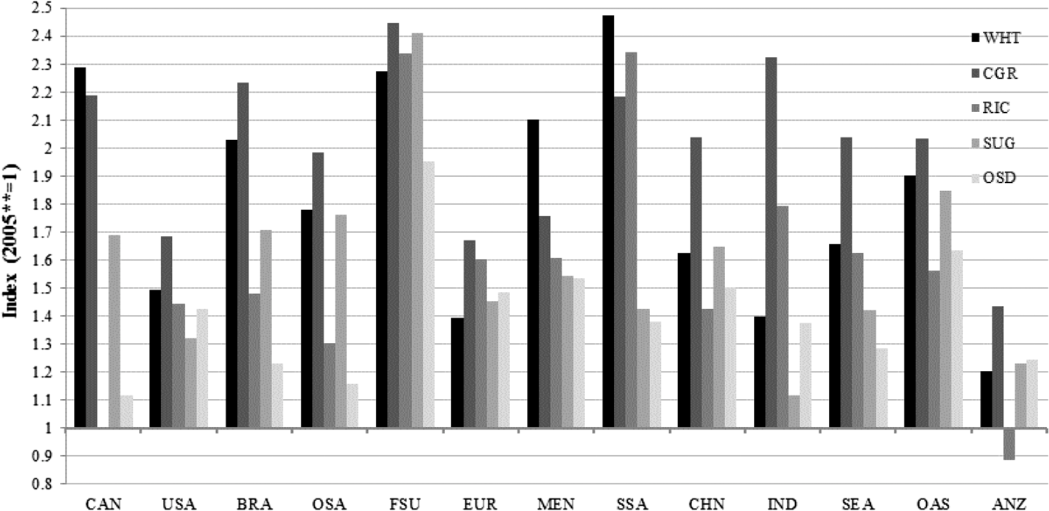

Figure 2 reports global price changes for agricultural aggregate across different AgMIP models. The price changes are heterogeneous across models ranging from a decline of 25% to an increase of 39% in 2050 relative to 2005. CAPRI alongside EPPA, FARM, MAGNET belong to the group of models which project a decline in agricultural prices in the long-term. The rest of models project an increase in prices over the same period. These differences in price projections are driven by a variety of factors such as differences in parameterization of models, agricultural land development, models’ response to macroeconomic developments, and differences in assumptions on the level of technical change of production factors.²⁹

Fig. 2

Price projections for the agricultural aggregate, 2005 to 2050. Global price growth index for agricultural aggregate in 2030 and 2050 relative to 2005 by AgMIP model.

Land use projections are also relatively heterogeneous in the reference scenario across models (Fig. 3). The change of total agricultural area, cropland, and pasture land varies between $- 2 %$ and 17%, $- 6 %$ and 26%, and $- 7 %$ and 14%, respectively, in 2050 relative to 2005. However, the projection of the expansion in the global land use tends to prevail across models. CAPRI reports an increase in land use for all three land categories reported in Fig. 3 similar to ENVISAGE, GTEM, MAGNET, GLOBIOM, IMPACT, and MAgPIE. Other models report mixed projections, out of which EPPA and FARM simulate a decrease in the total cultivated agricultural area. The variation in the projections across models are driven, among other things, by the type of data used to parameterize land allocation as well as by the approach applied to model mobility of land across different uses, agricultural land competition with other sectors and technological change.⁴⁵

Fig. 3

Area projections for the agricultural aggregate, cropland and pasture land, 2005 to 2050. Global area change for agricultural sector (AGR), cropland (CRP), and pasture (PAS) in 2050 relative to 2005 by AgMIP model.

3.2.

Climate Change Effects—Model Intercomparison

This section presents global results for four climate change scenarios and for 11 global economic models considered in AgMIP. Figure 4 reports model simulation results for the exogenous and endogenous effects of climate change on yields. Almost all models, with the exception of MAgPIE, consistently report a negative impact of climate change on yields relative to the reference scenario S1. The yield change in 2050 relative to the reference scenario lies between 20% and $- 25 %$ ; however, for most models and commodities the range is between $- 2 %$ and $- 15 %$ . GTEM generally has the smallest negative effects, whereas MAgPIE has the largest number of positive effects for some commodities. MAGNET shows the largest negative effects across all reported commodities.²² CAPRI projects negative-signed global agricultural yield responses across all four climate change scenarios and the effects tend to be at the lower range compared to other models but comparable to ENVISAGE, GTEM, and GLOBIOM.

Fig. 4

Global yield changes, (percentage change in 2050 relative to S1 in 2050). Percentage yield changes for climate change scenarios in 2050 relative to S1 in 2050 by commodity group and AgMIP model.

As a result of lower productivity, global agricultural prices increase relative to S1. The price increases range from 1.3% to 56% over the price in 2050 without climate change (Table 3). Globally, the scenarios using DSSAT results have greater price increases compared with the LPJmL scenarios. The GCAM, EPPA, and ENVISAGE models generally have the smallest price increases, whereas MAgPIE reports the largest positive price effects. Similar to other models, CAPRI projects an increase in the global producer prices in response to the predominantly adverse impacts of climate change on crop yields. The magnitude of the CAPRI simulated effects as well as the pattern across the four different impact scenarios is close to IMPACT, MAGNET, and AIM.²²^,²⁹^,³²

Table 3

Global price changes for agriculture aggregate, (percentage change in 2050 relative to S1 in 2050).

Models	S3	S4	S5	S6
AIM	5.5	6.6	11.5	10.8
ENVISAGE	2.8	3.2	3.3	3.5
EPPA	1.3	1.6	4.1	4.6
FARM	4.3	5.4	7.0	6.1
GTEM	4.9	6.0	6.7	6.2
MAGNET	10.6	11.0	13.5	14.7
GCAM	3.3	3.3	3.3	3.4
GLOBIOM	13.1	12.9	19.2	21.4
IMPACT	15.5	16.6	15.5	18.3
MAgPIE	7.7	56.5	29.8	51.2
CAPRI	11.2	12.5	10.6	13.2

Almost all models (with the exception of FARM) simulate an increase in the global agricultural area due to climate change. The area change varies between $- 0.2 %$ and 9.2% (Table 4). IMPACT and MAGNET have the largest agricultural area increases across the scenarios, whereas FARM, GLOBIOM, and MAgPIE report the smallest changes for most scenarios. The CAPRI projections are close to the median across all AgMIP models in all four climate scenarios.²²^,³²

Table 4

Global agricultural area changes (percentage change in 2050 relative to S1 in 2050).

Model	S3	S4	S5	S6
AIM	3.0	2.6	3.6	4.0
ENVISAGE	2.4	2.4	2.4	2.7
EPPA	0.9	0.7	2.1	2.1
FARM	$- 0.2$	$- 0.2$	$- 0.1$	0.1
MAGNET	4.6	4.4	6.4	6.9
GCAM	1.9	1.6	1.8	1.9
GLOBIOM	0.7	0.2	0.9	1.7
IMPACT	6.4	6.4	7.7	9.2
MAgPIE	0.5	0.6	1.2	1.6
CAPRI	1.3	1.1	1.1	1.2

4. Climate Change Impacts for China

This section presents climate change impacts for Chinese agriculture based on CAPRI simulation results. The exogenous yield shifters caused by the climate change show mixed results for China. For coarse grains and oilseeds, yields decrease in all four climate scenarios. For the rest of the crop groups, the climate change effects are mixed between positive and negative yield changes across scenarios.

The simulation results indicate a moderate impact of climate change on the Chinese agricultural prices at the aggregate AGR level. The aggregate prices increase between 4.7% and 5.2% relative to S1 without climate change (Table 5). These price effects are driven by the drop in global agricultural supply and changes in the Chinese production structure. However, there is strong variation across sectors; the sectoral prices change between 2.2% and 59% relative to the reference scenario (Table 5). A stronger price increase also occurs in 2050 relative to 2030 (not shown). The strongest price effect is observed for coarse grains and oilseeds and, for S5 and S6, also for wheat. Compared to other AgMIP models, the magnitude of the CAPRI results as well as their pattern across scenarios is close to the median. Models GLOBIOM, IMPACT, MAgPIE, and MAGNET report stronger price effects, whereas another cluster of models (ENVISAGE, GCAM, FARM, and GTEM) generate noticeably lower price impacts.²²^,²⁹^,³²

Table 5

CAPRI price changes for China (percentage change in 2050 relative to S1 in 2050).

Sector	S3	S4	S5	S6
AGR	5.2	5.7	4.7	4.7
CGR	18.7	17.3	47.1	43.7
DRY	4.8	4.9	10.6	9.8
NRM	5.0	5.3	6.7	6.6
OSD	19.4	13.2	22.1	23.4
RIC	24.5	24.3	11.2	9.5
RUM	6.6	6.8	14.8	13.5
SUG	2.2	2.6	2.6	3.2
WHT	4.2	8.3	59.0	49.5

The aggregate production drops on average between 0.4% and 3.3% relative to the reference scenario (Table 6). The S5 and S6 scenarios show stronger production decreases than the other two scenarios (S3 and S4) as well as stronger production increase that occurs in 2050 relative to 2030 (not shown). Looking at the sectoral disaggregated level we find stronger adjustments in the production, varying between 3% and $- 12.2 %$ relative to the reference scenario (Table 6). The highest decrease in production due to climate change is projected for coarse grains and oilseeds. On the other hand, wheat increases production in S3 and S4 and rice increases production in S5 and S6; these results are mainly driven by the differences in the climate induced yield changes. Compared to other AgMIP models, CAPRI projects the magnitudes of the production effects for China in line with AIM, ENVISAGE, FARM, and GTEM. Other AgMIP models tend to simulate considerably stronger climate change impacts on production.²²^,²⁹

Table 6

CAPRI production change results for China (percentage change in 2050 relative to S1 in 2050).

Sector	S3	S4	S5	S6
CGR	$- 2.9$	$- 2.6$	$- 12.2$	$- 10.3$
DRY	$- 0.2$	$- 0.3$	$- 1.2$	$- 1.0$
NRM	0.0	0.0	$- 0.8$	$- 0.6$
OSD	$- 0.4$	0.2	$- 5.2$	$- 3.0$
RIC	$- 0.7$	$- 0.3$	2.8	3.4
RUM	$- 0.3$	$- 0.4$	$- 2.4$	$- 2.0$
SUG	$- 0.7$	$- 0.7$	$- 1.3$	$- 1.0$
WHT	1.1	0.6	$- 5.7$	$- 4.6$
Averagea	$- 0.5$	$- 0.4$	$- 3.3$	$- 2.4$

^aSimple average.

Aggregate land use changes induced by climate change are relatively small. Relative to the reference scenario, the total agricultural area increases by 0.2% in scenarios S3 and S4 and by 0% in scenarios S5 and S6 (Table 7). Land relocation effects between different commodity aggregates are also relatively small; for most commodity aggregates it ranges between $- 5 %$ and 3%. A stronger climate change impact on land use is projected for coarse grains and wheat in scenarios S5 and S6. Land use for sugar decreases and for coarse grains it increases in all climate scenarios. These results are mainly driven by the relative changes in profitability of different crops caused by price and yields adjustments to climate change. For other crops, the results are mixed depending on the scenario (Table 7). The CAPRI area projections are somehow close to the median across all AgMIP models in all four climate scenarios.²²^,²⁹

Table 7

CAPRI area change results for China (percentage change in 2050 relative to S1 in 2050).

Sector	S3	S4	S5	S6
AGR	0.2	0.2	0.0	0.0
CGR	1.4	0.9	8.3	7.4
CR5	0.6	0.3	2.3	1.9
CRP	0.4	0.3	$- 1.2$	$- 0.9$
OSD	0.5	$- 0.3$	$- 4.4$	$- 3.5$
PAS	$- 0.1$	0.0	1.7	1.4
RIC	1.0	0.9	$- 4.8$	$- 4.3$
SUG	$- 1.9$	$- 2.0$	$- 5.2$	$- 4.4$
WHT	$- 2.4$	$- 1.3$	10.5	7.3

The reduced availability of agricultural commodities and higher prices due to climate changes is reflected in lower consumption levels dropping on average between 0.6% and 2.8% in China. The strongest effects are observed for coarse grains and wheat (Table 8). CAPRI-projected magnitudes of the consumption effects for China are in line with AIM, ENVISAGE, FARM, and GTEM. Other AgMIP models tend to simulate considerably stronger consumption responses to climate change.²²^,²⁹

Table 8

CAPRI consumption change results for China (percentage change in 2050 relative to S1 in 2050).

Sector	S3	S4	S5	S6
CGR	$- 3.5$	$- 3.0$	$- 12.3$	$- 11.1$
DRY	$- 0.3$	$- 0.3$	$- 1.3$	$- 1.1$
NRM	$- 0.2$	$- 0.2$	−0.9	$- 0.9$
OSD	$- 1.0$	1.3	0.4	2.1
RIC	$- 1.3$	$- 1.2$	0.4	0.5
RUM	$- 0.8$	$- 0.8$	$- 2.5$	$- 2.2$
SUG	$- 0.6$	$- 0.7$	$- 0.8$	$- 0.9$
WHT	0.8	0.3	$- 5.2$	$- 4.2$
Averagea	$- 0.9$	$- 0.6$	$- 2.8$	$- 2.2$

^aSimple average.

5. Discussion and Conclusions

The current paper investigates the long-term impacts of climate change on the global agriculture and the Chinese agriculture following the AgMIP approach. We provide horizontal model intercomparison for 11 AgMIP models as well as explore in more detail the application of the CAPRI modeling framework to systematically compare its performance with respect to other models and specifically for the Chinese agriculture. We compile one reference scenario which serves as a counterfactual situation for climate change scenarios. This scenario reflects economic assumptions as defined under the SSP2. We simulate four climate change scenarios. All scenarios are run for 2030 and 2050.

The long-term projections of agricultural productivity in the reference scenario without climate change show relatively robust but heterogeneous growth across commodity groups. Overall, the exogenous productivity change varies between 20% and 100% in 2050 relative to 2005. There is no consensus in price and area projections across models in the reference scenario; this is the case for both the magnitude and the sign of the projected changes. The aggregate price changes at the global level range from a decline of 25% to an increase of 39% in 2050 relative to 2005. The projected change for the total agricultural area varies between $- 2 %$ and 17%.

In general, there are relatively moderate effects of climate change at the global level. The results indicate that, at the global level, the climate change will cause a decrease in the agricultural productivity between $- 2 %$ and $- 15 %$ by 2050. The productivity decline will in turn generate upward pressure on global food prices (between 1.3% and 56%) and will lead to expansion of cultivated area (between 1% and 4%) over the same period. However, there is a stronger impact across different agricultural commodities. Sectoral impacts of climate change may increase by a factor higher than 5 or more relative to the aggregate global impacts.

The model intercomparison for climate change scenarios shows relatively strong heterogeneity in the simulated effects between models. Although all models tend to report consistently higher prices, lower yields, increase in area use, and reduction in consumption as a response to climate change, the strongest differences between models are in the relative magnitude of the simulated effects.

The analyses of this paper show that the CAPRI simulations are in line with (or within the variation of) the rest of the AgMIP models. The most significant differences are observed for price projections for the reference scenario where CAPRI reports a decline in prices which is consistent with three CGE models (EPPA, FARM, MAGNET) but is in conflict with all PE models. The results for China are in line with the general projections for the global agriculture with the difference that the climate change effects (e.g., yield decrease and price increase) tend to be smaller. The analyses for the Chinese agriculture also reveal that CAPRI projections are close to the median across all AgMIP models.

Overall, the analyses conducted in this paper revealed that the main discrepancy in simulated effects across models occurred for the reference scenario. For this scenario, the differences in projections differ not only in the magnitude but also in the direction (sign) of the simulated changes. For the climate change scenarios, the signs of the changes are broadly in line across models, whereas the magnitudes can vary substantially; sometimes the differences could be more than fivefold large.

Key sources of differences in simulated effects are the model type (i.e., PE versus CGE model) and how trade flows are modeled. For example, for price effects, the PE models appear to produce systematically higher price changes as compared to the CGE models. This is most likely because CGE models generally consider greater degrees of substitution within the production and demand systems as well as including non-AGRs, implying that a part of the effects occurring in agriculture might be absorbed by non-AGRs. The differences in results between CGE and PE models could also partially be explained by how the climate change is modeled. In CGE models, climate change shocks are introduced by adjusting the land efficiency parameter in the production function, whereas in PE models the shocks are reflected by adjusting crop yields or supply functions. Further, models with spatially explicit representation of bilateral trade flows (e.g., Armington approach) tend to result in smaller price increases in the reference scenario and larger increases in the climate change scenarios than other models. These results are contradictory and require further research. The theoretical hypothesis would suggest a lower price transmission in models with spatially explicit modeling of trade flows resulting in stronger price adjustment to exogenous shocks due to the implicit assumption of more segmented markets.²²^,²⁹

A second factor that causes divergence in the simulated effects across models is income and the price elasticities of food demands. These elasticities are behavioral parameters which measure responsiveness of the food quantity demanded to income and price changes. They determine the magnitude of adjustments taking place in the AGR as a response to changes occurring in the macroeconomy (e.g., GDP growth) or on the supply side of the AGR (e.g., due to climate change). The differences in elasticities between models are relatively significant causing heterogeneity in the simulated effects. For example, contrary to expectation, some models has elasticities increasing over time (e.g., ENVISAGE, AIM), whereas others have theoretically consistent decreasing elasticities over time for most commodity groups (e.g., CAPRI, GLOBIOM, IMPACT) causing a strong differences in agricultural market responses across models to GDP growth in the reference scenario and to productivity changes in the climate scenarios.²²^,²⁹

The third reason for the differences in model results relates to the unavailability of accurate primary and secondary economic data on issues linked, for example, to agricultural land use, technological change, and costs of primary production factors. The fourth cause for differences could be associated with a need to better reflect interdisciplinary knowledge into economic models, in particular, those linked to biophysical relationships and interactions. This shortcoming is particularly visible from the relatively large discrepancy in simulated land use developments. The land use response is fundamental in determining the potential for expansion or contraction of agricultural production at the extensive margin, which can have an offsetting effect on the climate change induced impacts at the intensive margin of the agricultural production (i.e., through yield changes).²²^,²⁹

The analysis of CAPRI performance reveals that its simulated effects are, in general, close to the median across all AgMIP models. CAPRI contains some specific features which are either not considered in the rest of the PE models or are treated differently depending on the model component. First, CAPRI is an exception across all PE models as it models trade flows using the Armington approach, which is considered only in CGE models. Second, CAPRI models climate change by applying a different approach in the supply module than in the market module. Most other models usually use only one approach. In the market module, CAPRI parameters of supply functions are adjusted, whereas in the supply module, crop yields are adjusted. Given that CAPRI combines elements from different models (including from CGE), this may partly explain why the CAPRI results tend to lie at the mid-point across AgMIP models.

The analyses of this paper also reveal that there are substantial differences in projections of climate change impacts across scenarios determined by circulation models and crop models. The differences in simulated effects between scenarios tend to be consistent across the 11 economic models, but often exceed the differences in the simulated effects between the models. Model intercomparison studies done for crop models within the AgMIP project show that the model uncertainties of the climate induced yield changes can be substantial. The climate change impacts across crop models vary depending on the model structure and parameter values. These studies also suggest that a relatively small set of well-defined models can quantify the model uncertainty relatively accurately and in some cases substantially reduce the variability.⁴⁶^–⁴⁸ Applying this work in economic modeling may result in more accurate quantification of the uncertainty of economic effects of climate change as well as it may deliver less uncertain results. This would be a promising avenue for future research as it would contribute to a better understanding of uncertainties of AGR responses to climate change from an interdisciplinary point of view.

An issue that may require further consideration is the responsiveness of fodder production to climate change. In this assessment, yields of fodder crops including grasslands have not been varied in the climate change scenarios, mainly because fodder crops are not explicitly included in the product list of the IMPACT model that served to compile the standardized productivity shocks. Yet it may be expected that fodder crops would be just as vulnerable to climate impacts as other crops. Including assumptions on such effects would considerably reinforce the global market effects via the animal sector.

Acknowledgments

The authors would like to thank Dirk Willenbockel for very helpful comments on the CAPRI results and Gerald Nelson for coordination and contribution to the AgMIP model intercomparisons. The authors are solely responsible for the content of the paper. The views expressed are purely those of the authors and may not in any circumstances be regarded as stating an official position of the European Commission.

References

1.

G. C. NelsonD. BereuterD. Glickman, “Advancing global food security in the face of a changing climate,” (2014). Google Scholar

2.

W. E. Easterlinget al., “Agricultural impacts of and responses to climate change in the Missouri-Iowa-Nebraska-Kansas (MINK) region,” Clim. Change, 24 (1–2), 23 –61 (1993). http://dx.doi.org/10.1007/BF01091476 CLCHDX 0165-0009 Google Scholar

3.

D. R. Peiriset al., “A simulation study of crop growth and development under climate change,” Agric. For. Meteorol., 79 (4), 271 –287 (1996). http://dx.doi.org/10.1016/0168-1923(95)02286-4 0168-1923 Google Scholar

4.

K. Hakala, “Growth and yield potential of spring wheat in a simulated changed climate with increased CO2 and higher temperature,” Eur. J. Agron., 9 (1), 41 –52 (1998). http://dx.doi.org/10.1016/S1161-0301(98)00025-2 EJAGET 1161-0301 Google Scholar

5.

R. MendelsohnA. Dinar, Climate Change and Agriculture: An Economic Analysis of Global Impacts, Adaptation and Distributional Effects, Edward Elgar Publishing, Cheltenham, United Kingdom (2009). Google Scholar

6.

M. L. Parryet al., “Effects of climate change on global food production under SRES emissions and socio-economic scenarios,” Global Environ. Change, 14 (1), 53 –67 (2004). http://dx.doi.org/10.1016/j.gloenvcha.2003.10.008 GCHRE2 Google Scholar

7.

R. A. BrownN. J. Rosenberg, “Climate change impacts on the potential productivity of corn and winter wheat in their primary United States growing regions,” Clim. Change, 41 (1), 73 –107 (1999). http://dx.doi.org/10.1023/A:1005449132633 CLCHDX 0165-0009 Google Scholar

8.

V. CuculeanuA. MarciaC. Simota, “Climate change impact on agricultural crops and adaptation options in Romania,” Clim. Res., 12 153 –160 (1999). http://dx.doi.org/10.3354/cr012153 CLREEW 0936-577X Google Scholar

9.

G. Piroliet al., “From a rise in B to a fall in C? Environmental impact of biofuels,” Economics and Econometrics Research Institute (EERI), Brussels (2014). Google Scholar

10.

S. Shresthaet al., “Impacts of climate change on EU agriculture,” Rev. Agric. Appl. Econ., 16 (2), 24 –39 (2013). Google Scholar

11.

R. M. Adamset al., “The economic effects of climate change on U.S. agriculture,” The Economics of Climate Change, 18 –54 Cambridge University Press, Cambridge (1998). Google Scholar

12.

R. Darwinet al., “World agriculture and climate change: economic adaptations,” (1995). Google Scholar

13.

“Chapter 7 Food Security and Food Production Systems,” (2014). Google Scholar

14.

A. GhaffariH. F. CookH. C. Lee, “Climate change and winter wheat management: a modelling scenario for south eastern England,” Clim. Change, 55 509 –533 (2002). http://dx.doi.org/10.1023/A:1020784311916 CLCHDX 0165-0009 Google Scholar

15.

P. G. JonesP. K. Thornton, “The potential impacts of climate change on maize production in Africa and Latin America in 2055,” Global Environ. Change, 13 (1), 51 –59 (2003). http://dx.doi.org/10.1016/S0959-3780(02)00090-0 GCHRE2 Google Scholar

16.

F. I. WoodwardG. B. ThompsonI. F. McKee, “How plants respond to climate change: migration rates, individualism and the consequences for plant communities,” Ann. Bot., 67 (Supp 1), 23 –38 (1991). ANBOA4 0305-7364 Google Scholar

17.

G. R. Battset al., “Effects of CO2 and temperature on growth and yield of crops of winter wheat over four seasons,” Eur. J. Agron., 7 (1–3), 43 –52 (1997). http://dx.doi.org/10.1016/S1161-0301(97)00022-1 EJAGET 1161-0301 Google Scholar

18.

J. I. L. MorisonD. W. Lawlor, “Interactions between increasing CO2 concentration and temperature on plant growth,” Plant Cell Environ., 22 (6), 659 –682 (1999). http://dx.doi.org/10.1046/j.1365-3040.1999.00443.x PLCEDV 1365-3040 Google Scholar

19.

R. S. J. Tol, “The economic effects of climate change,” J. Econ. Perspect., 23 (2), 29 –51 (2009). http://dx.doi.org/10.1257/jep.23.2.29 0895-3309 Google Scholar

20.

“Impacts, Adaptation and Vulnerability,” (2007). Google Scholar

21.

“Impacts, Adaptation and Vulnerability,” (2014). Google Scholar

22.

G. C. Nelsonet al., “Agriculture and climate change in global scenarios: why don’t the models agree,” Agric. Econ., 45 (1), 1 –18 (2014). http://dx.doi.org/10.1111/agec.2014.45.issue-1 1574-0862 Google Scholar

23.

G. C. Nelsonet al., “Climate change effects on agriculture: economic responses to biophysical shocks,” Proc. Natl. Acad. Sci., 111 (9), 3274 –3279 (2014). http://dx.doi.org/10.1073/pnas.1222465110 PMASAX 0096-9206 Google Scholar

24.

M. von LampeD. WillenbockelG.C. Nelson, “Overview and key findings from the global economic model comparison component of the Agricultural Intercomparison and Improvement Project (AgMIP),” in 16th Int. Conf. on Global Economic Analysis, (2013). Google Scholar

25.

J. C. Ciscaret al., “Climate impacts in Europe: the JRC PESETA II project,” (2014). http://dx.doi.org/10.2791/7409 Google Scholar

26.

A. Gochtet al., “Farm type effects of an EU-wide direct payment harmonisation,” J. Agric. Econ., 64 (1), 1 –32 (2013). http://dx.doi.org/10.1111/1477-9552.12005 1068-5502 Google Scholar

27.

A. Leipet al., “Farm, land, and soil nitrogen budgets for agriculture in Europe calculated with CAPRI,” Environ. Poll., 159 (11), 3243 –3253 (2011). http://dx.doi.org/10.1016/j.envpol.2011.01.040 ENPOEK 0269-7491 Google Scholar

28.

M. Kempenet al., “Economic and environmental impacts of milk quota reform in Europe,” J. Policy Modell., 33 (1), 29 –52 (2011). http://dx.doi.org/10.1016/j.jpolmod.2010.10.007 0161-8938 Google Scholar

29.

V. von Lampeet al., “Why do global long-term scenarios for agriculture differ? An overview of the AgMIP Global Economic Model Intercomparison,” Agric. Econ., 45 (1), 1 –18 (2014). http://dx.doi.org/10.1111/agec.2014.45.issue-1 1574-0862 Google Scholar

30.

S. Robinsonet al., “Comparing supply-side specifications in models of global agriculture and the food system,” Agric. Econ., 45 (1), 1 –15 (2014). http://dx.doi.org/10.1111/agec.2014.45.issue-1 1574-0862 Google Scholar

31.

H. Valinet al., “The future of food demand: understanding differences in global economic models,” Agric. Econ., 45 (1), 1 –17 (2014). http://dx.doi.org/10.1111/agec.2014.45.issue-1 1574-0862 Google Scholar

32.

D. Willenbockel, “Comparison and integration of CAPRI scenario results in the AgMIP global economic model track project,” (2013). Google Scholar

33.

B. C. O’Neillet al., “Workshop on the nature and use of new socioeconomic pathways for climate change research,” in Meeting Report, National Center for Atmospheric Research (NCAR), (2011). Google Scholar

34.

E. Kriegleret al., “The need for and use of socio-economic scenarios for climate change analysis: a new approach based on shared socio-economic pathways,” Global Environ. Change, 22 (4), 807 –822 (2012). http://dx.doi.org/10.1016/j.gloenvcha.2012.05.005 GCHRE2 Google Scholar

35.

D. P. Van Vuurenet al., “Scenarios in global environmental assessments: key characteristics and lessons for future use,” Global Environ. Change, 22 (4), 884 –895 (2012). http://dx.doi.org/10.1016/j.gloenvcha.2012.06.001 GCHRE2 Google Scholar

36.

P. Havlíket al., “Global land-use implications of first and second generation biofuel targets,” Energy Pol., 39 (10), 5690 –5702 (2011). http://dx.doi.org/10.1016/j.enpol.2010.03.030 ENPYAC Google Scholar

37.

G. Nelsonet al., Food security, farming, and climate change to 2050: scenarios, results, policy options, International Food Policy Research Institute, Washington, DC (2010). Google Scholar

38.

R. H. Mosset al., “The next generation of scenarios for climate change research and assessment,” Nature, 463 747 –756 (2010). http://dx.doi.org/10.1038/nature08823 NATUAS 0028-0836 Google Scholar

39.

C. MullerR. Robertson, “Projecting future crop productivity for global economic modeling,” Agric. Econ., 45 (1), 37 –50 (2014). http://dx.doi.org/10.1111/agec.2014.45.issue-1 1574-0862 Google Scholar

40.

D. Schimmelpfenniget al., “Agricultural adaptation to climate change: issues of long-run sustainability,” (1996). Google Scholar

41.

R. M. Adamset al., “Effects of global climate change on agriculture: an interpretative review,” Clim. Res., 11 19 –30 (1998). http://dx.doi.org/10.3354/cr011019 CLREEW 0936-577X Google Scholar

42.

F. J. Fernándezet al., “Still a challenge—interaction of biophysical and economic models for crop production and market analysis,” (2013). Google Scholar

43.

W. BritzP. Witzke, “CAPRI model documentation 2012,” (2012). Google Scholar

44.

P. S. Armington, “A theory of demand for products distinguished by place of production,” IMF Staff Papers, 16 (1), 159 –176 (1969). http://dx.doi.org/10.2307/3866403 1020-7635 Google Scholar T. JanssonT. Heckelei, “Estimating a primal model of regional crop supply in the European Union,” J. Agric. Econ., 62 (1), 137 –152 (2011). http://dx.doi.org/10.1111/jage.2011.62.issue-1 1068-5502 Google Scholar

45.

S. Schmitzet al., “Land-use change trajectories up to 2050: insights from a global agro-economic model comparison,” Agric. Econ., 45 (1), 1 –16 (2014). http://dx.doi.org/10.1111/agec.2014.45.issue-1 1574-0862 Google Scholar

46.

S. Assenget al., “Uncertainty in simulating wheat yields under climate change,” Nat. Clim. Change, 3 827 –832 (2013). http://dx.doi.org/10.1038/nclimate1916 NCCACZ 1758-678X Google Scholar

47.

S. Bassuet al., “How do various maize crop models vary in their responses to climate change factors?,” Global Change Biol., 20 (7), 2301 –2320 (2014). http://dx.doi.org/10.1111/gcb.12520 1354-1013 Google Scholar

48.

T. Liet al., “Uncertainties in predicting rice yield by current crop models under a wide range of climatic conditions,” Global Change Biol., (2014). http://dx.doi.org/10.1111/gcb.12758 1354-1013 Google Scholar

Biography

Jacques Delincé is senior researcher and head of the unit of the Agriculture and Life Sciences in the economy unit at the Joint Research Centre (JRC) of the European Commission.

Pavel Ciaian is senior researcher at the Joint Research Centre (JRC) of the European Commission.

Heinz-Peter Witzke is senior researcher at the Institute for Food and Resource Economics at the Bonn University.

CC BY: © The Authors. Published by SPIE under a Creative Commons Attribution 4.0 Unported License. Distribution or reproduction of this work in whole or in part requires full attribution of the original publication, including its DOI.

Citation Download Citation

Jacques Delincé, Pavel Ciaian, and Heinz-Peter Witzke "Economic impacts of climate change on agriculture: the AgMIP approach," Journal of Applied Remote Sensing 9(1), 097099 (21 January 2015). https://doi.org/10.1117/1.JRS.9.097099

Published: 21 January 2015

Access the abstract

JOURNAL ARTICLE
16 PAGES

DOWNLOAD PAPER SAVE TO MY LIBRARY

GET CITATION

CITATIONS

Cited by 19 scholarly publications.

Explore citations on Lens.org

KEYWORDS

Climate change

Agriculture

Climatology

Data modeling

Atmospheric modeling

Systems modeling

Performance modeling

1.

Introduction

2.

Methodology