
|
|
1.IntroductionLeaf area index (LAI), defined as the one-sided green leaf area per unit ground surface area,1 is used as one key parameter for surface modeling of hydrological processes, ecological development, and global change.2–4 Remote sensing uses physical and empirical models to estimate LAI;5–7 however, the physical models are usually complex and the parameter inversions do not always converge. The simpler empirical models are usually adopted for various applications,8,9 but empirical models are site-specific and vary with sensor configuration. This variation is because the reflectance of forest canopy is affected by many factors such as soil and atmospheric conditions, sensor viewing geometry, and vegetation type,10 and differences in understory structure and percent canopy cover are also important factors on canopy reflectance.11,12 Therefore, it is important to understand the effects of these factors on the precision of the LAI estimation. LAI has been successfully estimated from remote sensing data for different species such as wheat (Triticum),13 oats (Avena sativa),14 corn (Zea mays),15 and cotton (Gossypium hirsutum).16 Other communities like grass,17 shrub,18 and forest19 have also appeared frequently in literature. The spatial homogeneity of crops and shrub-grasses allows the empirical models (linear or nonlinear) to yield higher accuracy in LAI estimation when compared with forests, characterized by complicated structures.20 Biochemical characteristics of different species also play an important role in LAI-VI response.21,22 Colombo et al.8 concluded that the LAI-VI models were better for vineyard, soybean, corn, and poplar plantations () than for native forests (). Gu et al.23 found that the LAI-VI models were more accurate for planted trees than for native forests with increased biodiversity and complex structures. Traditional LAI estimation was mostly conducted using data acquired from a near nadir position, such as the Landsat24 and the Systeme Probatoire d’Observation de la Terre,25 on both local and regional areas worldwide. Differences in viewing geometry (both view and illumination angles) have been ignored in most of these studies. Some studies treated it as a source of uncertainty, and methods were devised to correct the angle effect using either a simple empirically derived cosine technique26 or the bidirectional reflectance distribution function models.27 Others tried to use the angle to derive information of the anisotropic characteristics of the target. Diner et al.28 and Yao et al.29 confirmed that compared with the monoangular observation, the use of the multiangular data can improve the potentials of VIs in LAI estimation. The multiangular observation contains more information about the anisotropic characteristics of the vegetation structures and influences of canopy shadows. Many traditional VIs like normalized difference vegetation index (NDVI), soil adjusted vegetation index (SAVI), and global environmental monitoring index (GEMI) were shown to perform differently at various observation angles.26,30,31 Verrelst et al.32 used the Compact High-Resolution Imaging Spectrometer onboard the Project for On-board Autonomy (CHRIS/PROBA) imagery to derive several VIs for evergreen coniferous forests and meadows. The influence of observation angles on the equations for most of the indices was found to differ with vegetation type, which provides an additional means for the inversion of vegetation structures. VIs have been designed as a proxy to quantify the vegetation33 and reduce the effects of nonvegetation factors.34 Earlier VIs were usually linear combinations (subtraction or summation) in addition to ratios of primary bands such as NDVI35 and simple ratio index.36 Many studies have demonstrated a strong correlation between such indices and LAI;37 however, the correlation was influenced by the soil background, especially on sparsely vegetated areas. To reduce the soil background effect, Richardson and Wiegand38 proposed the perpendicular vegetation index (PVI) using the concept of soil line. Huete39 suggested, instead, that the PVI is still affected by the optical properties of the soil background. Following this suggestion, the SAVI was analyzed by Purevdorj et al.40 using the soil adjustment factor determined by soil background variations. For example, was found to perform well for moderately dense vegetation. Furthermore, Baret et al.41 proposed the transformed SAVI (TSAVI) by taking into account the soil line slope and intercept. Qi et al.42 used the modified SAVI (MSAVI), which replaces the constant with a dynamic , making the adjustment of the soil background effect more scene specific. The atmospheric effects have consistently been a concern in the calculation of VIs. The atmospherically resistant vegetation index (ARVI),43 using the radiation of the blue channel to correct the atmospheric effects, improved LAI estimation accuracy.23 Given that the soil and atmosphere affect the radiation simultaneously, Huete et al.44 proposed the enhanced vegetation index, integrating SAVI and ARVI in the index. In hyperspectral and thermal infrared remote sensing, narrow-band VIs were widely experimented with. Brantley et al.45 concluded that the red edge indices performed LAI estimation more accurately than broadband indices, such as NDVI and ratio vegetation index (RVI), when LAI is greater than 4. In brief, vegetation type, data acquisition geometry, and index design may inherently influence the reliability of LAI estimation; however, the systematic analysis of these influences was rarely documented. The objective of this study is to analyze the predictability of LAI-VI modeling to variations in three factors: vegetation type, the observation angle, and the VI. To achieve this: (1) LAIs were measured in situ for different vegetation communities, and related VIs were derived from different observation angles from CHRIS/PROBA imagery data; and (2) LAI-VI models were established for each vegetation-angle-index combination followed by an assessment of the performance of the models for each of the three factors. 2.Materials and Methods2.1.Study Area and Data SourceThe study area (Fig. 1) is located in Yugan County in Jiangxi Province, China (E116°29′46′′–116°33′24′′, N28°42′52′′–28°49′19′′). A subtropical humid monsoon climate dominates the area, with a mean annual temperature of 17.8°C and a mean annual precipitation of 1586.4 mm. The majority of rainfall occurs from April to June. Landforms primarily include rolling hills and lakeside plains, with an altitude of about 150 to 250 m above sea level. Forest coverage is about 20.5% and the remaining landscape consists mainly of shrub and grasslands. Sample sites are located in hilly regions with a slope of less than 15 deg. Fig. 1Location of the study area (a) and false color composition (b) of the CHRIS/PROBA data acquired on May 11, 2008. The composition was produced with , , and . The white circles on (b) mean the sampling sites.  Remotely sensed images were retrieved from the CHRIS/PROBA data. The CHRIS sensor provides coregistered images with a spatial resolution of 17 m (pixel size) over the spectral range 415 to 1050 nm. PROBA is an experimental platform which enables the sensor to capture images from five viewing angles, nominally , , and 0 deg.46 CHRIS Mode 332,47 data were acquired over the study area on May 11, 2008, under nearly cloud-free conditions (Table 1). Solar position was assumed to be constant given that the time difference between the images sequences was less than 2 min. For convenience, the image sequences before the nadir ( and ) and after the nadir ( and ) are also referred to as forward and backward series, respectively. Table 1CHRIS image acquisition and illumination geometry from May 11, 2008. Acquisition time is the Universal Time Coordinated (UTC) on the image acquisition day in the format of HH:MM:SS.
2.2.Leaf Area Index Field MeasurementTwenty-five field sampling sites were deployed in locations with undisturbed natural vegetation over the sampling period,48 taking the typical vegetation types and accessibility into consideration. Four plots ( sized) were located within each site. A total of 100 plots were sampled: 26, 21, 30, 12, and 11 for grass (GR), shrub (SH), coniferous forest (CF), coniferous and broad leaf forest (CB), and broad leaf forest (BF), respectively. The main vegetation species are: GR—Zephyranthes grandiflora, Zephyranthes candida, and Fatsia japonica; SH—Rosa chinensis Jacq, Camellia japonica L., Photinia glabra, and Thevetia peruviana; CF—Pinus thunbergii Parl., Podocarpus macrophyllus, and Pinus massoniana; and BF—Schima superba, Cinnamomum camphora, Elaeocarpus apiculatus Mast, and Sapium discolor. All plots were configured more than 30 m far away from each other to avoid overlap of the corresponding image pixels. The characteristics of vegetation on field measured sites are shown in Table 2. Tree heights were obtained by calculating the horizontal viewer-trunk distance and the viewer’s elevation angle of the tree top as measured with a tree height gauge. Tree canopy height means tree height minus canopy bottom height measured in the same way as the tree height. Radii of the tree canopy crown were measured with a laser distance detector by randomly choosing four points along the vertically projected “column” of the canopy and measuring and averaging their horizontal distances to the trunk. The fractional cover of vegetation (VFC) was measured using the photography method suggested by Gu et al.49 The precise locations of the plots were determined within an error of 1 m using a Starlink Invicta™ 210 Global Positioning System (GPS) receiver (RAVEN Industries, Inc., USA). LAI measurements were taken in early May 2010 under diffuse radiation conditions of overcast sky. The two-year difference between field and satellite data was addressed by carefully selecting plots with no change to vegetation type and coverage within that period. Two LAI-2000 Plant Canopy Analyzers (Li-COR, Lincoln, Nebraska) were operated in remote data acquisition mode, one used for reference readings (sky) and positioned in an open area proximal to the sampling site, and the other used in each plot to measure light transmission through the canopy. The under-canopy measurements were taken at about a 1 m height for forests and on the ground for shrubs and grasses. Both LAI analyzers were covered with a 270-deg view cap. About 5 to 8 below-canopy measurements were taken every 2 to 3 m along two parallel transects spaced by 10 m. The below-canopy measurements were compared with the above-canopy readings and the LAI was calculated and averaged for each plot. Table 2Characteristics of vegetation on field measured site.a
2.3.Image Preprocessing and Vegetation Index DerivationCHRIS products were provided with the radiometrically calibrated top of the atmosphere (TOA) radiance, and they were affected by both random and partially deterministic disturbances.32 The multiangular CHRIS observations introduce strong perspective distortions, especially for larger observation angles (). Consequently, the noise reduction, cloud screening, atmospheric correction, and geometric correction were carried out for image preprocessing using the software BEAM, a toolbox distributed by the European Space Agency (ESA). The noise reduction tool was used to correct dropouts and vertical striping on the image. Cloudy pixels were masked using the cloud screening tool. The TOA radiance was then converted to at-surface reflectance via the atmospheric correction tool using the water vapor data provided by ESA for CHRIS acquisition mode 3. Compared with the digital numbers, the corrected spectra of three typical land covers indicated that the atmospheric correction improves the differentiation of typical land covers, but still overperforms for the last four bands (863 to 1035 nm), a known issue of CHRIS data processing using BEAM;50 therefore, these bands were removed from the analysis of this study. Lastly, image georectification was completed through a coordinate map, aided by 15 field acquired ground control points. All the CHRIS bands were rectified to the WGS-84 coordinate system. To derive VIs for each in situ measurement from CHRIS data, a 20-m buffer around each plot center was used under the WGS-84 coordinate system. The average value of each band within the buffer was used for further analysis and VI calculation. Correlation coefficients between measured LAI and reflectance of each band were computed and compared. Reflectance values of three bands, band 3 (green, 530 nm), 8 (red, 672 nm), and 14 (near-infrared, 781 nm), have a strong correlation with LAI and typical spectral characteristics of corresponding visible/near-infrared ranges, so these were selected for VI derivation. Five commonly used VIs were calculated including NDVI,35 RVI,51 PVI,38 MSAVI,42 and modified chlorophyll absorption ratio index (MCARI2).52 These VIs represent three groups: traditional ratio-based (NDVI and RVI), soil-adjusted (PVI and MSAVI), and other visible light band besides red and near-infrared bands involved (MCARI2, referred to as multiple bands involved VI hereafter for easy description). The VIs are calculated by Eqs. (1)–(5), respectively: where NIR, RED, and GREEN are the reflectances of the near-infrared (781 nm), red (672 nm), and green (530 nm) bands, respectively. The soil line included in the above equations was from the references, but not from our data, because only marginal variations were found among the parameters shown above after plotting the soil line with some limited (and possibly not so typical) bare soil pixels from the image. The VIs were derived for five observation angles, which are hereafter referred to as 0 deg NDVI, 36 deg NDVI, and so on.2.4.LAI-VI Modeling and Predictability AnalysisLAI-VI models were first established with modeling data. After sorting plot LAIs of each vegetation type in ascending order, plot data were first divided into two independent subsets: modeling (M) and validation (V), in “MVMVM” cycling sequence, yielding in total 60 and 40 plots for modeling and validation, respectively. Quadratic polynomial regression models, for their simple and nonlinear performance, were established between LAIs and VIs for each vegetation type. Model performance was assessed through the determination coefficient () and mean relative error (MRE). The MRE was calculated using where , , and are the model estimated LAI, field measured LAI of plot , and the number of validation samples, respectively.Many predictability (or sensitivity in some literature) analysis methods in LAI estimation were used in literature, such as direct comparison of LAI-VI linear models,53 calculating the noise equivalent parameter22,54 and averaging VIs from different observation angles.55 The standard deviation of the variables (e.g., VI or model ) was also used in predictability studies.56 Gu et al.57 analyzed the influence of the radiometric correction level, VI, and polynomial power choice on VFC-VI modeling using the standard deviation of model values. Similarly in this paper, to evaluate the predictability of LAI-VI models to variations in vegetation type, observation angle, and VI, the standard deviation of for each of the three factors was calculated when the other two factors were fixed. For example, in the estimation of grass LAI using nadir observation data, the standard deviation of for five models established between LAI and five VIs indicates the model predictability to the variation of VIs in such GR 0 deg combination. An increased standard deviation indicates an increase in the predictability. They were hereafter called predictability to the variation of vegetation type (PVGT), observation angle (PANG), and VI (P-VI, to be different from the VI of PVI), respectively. To further compare the predictability and applicability of angle-index combinations in LAI estimation, multivariable-based linear regression models were established using the stepwise regression method with 25 variables () for each vegetation type. Statistical analyses of the predictability were performed using the software Statistical Product and Service Solutions (SPSS), version 19.0 (SPSS Inc., USA). 3.Results and Discussion3.1.LAI-VI Relationship ModelsThe determination coefficients () of the quadratic polynomial regression models for CB, BF, and GR were generally high and clustered (Fig. 2), but were relatively low and scattered for CF and SH, indicating that the soil background due to low LAI of these two vegetation types (Table 2) greatly influenced the modeling. There is an overall strong negative correlation between MREs and (, ) of all LAI-VI models, but interestingly, only coniferous forest shows a significant correlation (, ). The values seem to differentiate the vegetation communities much better than MRE, so this section will deal exclusively with values. Fig. 2Determination coefficient () and its relationship with mean relative error (MRE) of the leaf area index-vegetation index (LAI-VI) quadratic polynomial regression models for vegetation types of grass (GR), shrub (SH), coniferous forest (CF), coniferous and broad leaf forest (CB), and broad leaf forest (BF). 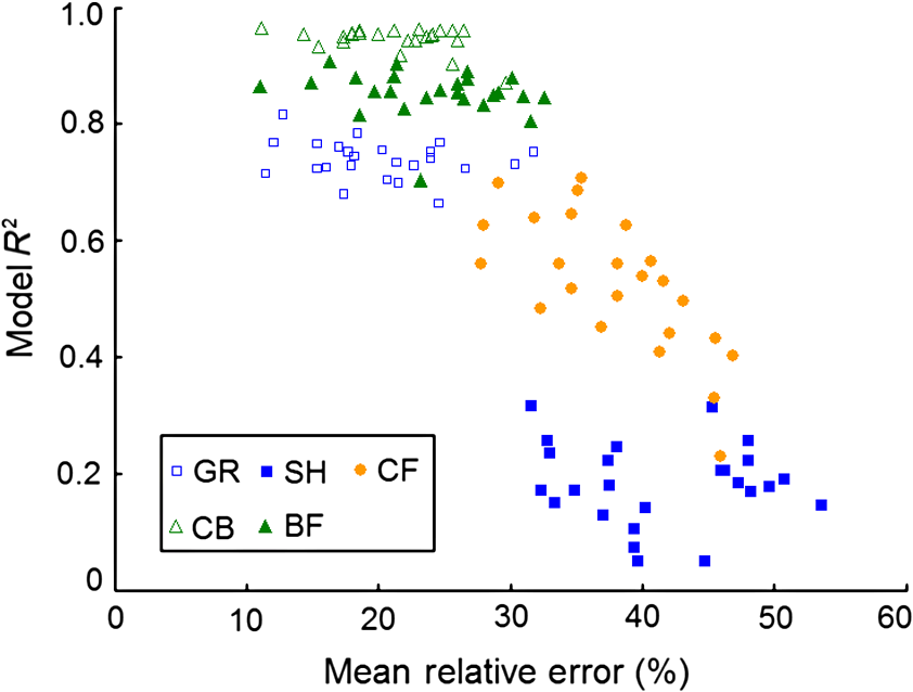 The comparison of the model determination coefficients suggested that LAI-VI models for forests with broad leaf trees are better than for relatively sparse vegetation including CF and SH (Table 2). The reliability of the models demonstrated by both and MRE values indicates that the LAI-VI models perform quite differently for different vegetation-angle-index combinations, which inspires the predictability analysis for better variable selection in the modeling. 3.2.Predictability Analysis of the ModelThe predictabilities are generally ranked as (Fig. 3). Model predictabilities to each of the three factors (vegetation, angle, and index) are analyzed and compared in the following sections. Fig. 3The predictability of LAI-VI quadratic polynomial regression models over three factors: (a) vegetation type (PVGT), (b) observation angle (PANG), and (c) vegetation index (P-VI). 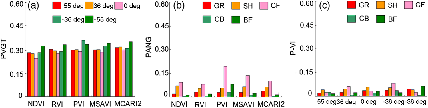 3.2.1.Vegetation typePVGT differs greatly with the combination of observation angle and VI [Fig. 3(a)]. The greatest PVGT is found at PVI (0.365) and the smallest at 0 deg NDVI (0.248). This suggests that the extreme PVGTs occur on the two less oblique observation angles. For each observation angle, the average PVGT of models shows , indicating that the models based on all oblique observation angles are more predictable to the variation of vegetation type than the traditional nadir observation, especially on the backward series ( and ). For each VI, the average PVGT of the models shows , indicating that VIs considering the green band besides conventional red and near-infrared bands (MCARI2) or indices accounting for soil background effects (PVI and MSAVI) are more predictable to the variation of vegetation types in LAI estimation. 3.2.2.Observation angleThe greatest PANG is found for CF PVI (0.195), and the least, CB MCARI2 (0.004), indicating that the extreme PANGs occur only for forests with coniferous trees [Fig. 3(b)]. For each vegetation type, the average PANG (in order) is . This demonstrates that both vegetation density and architecture influence such predictability: the sparse CF and SH yield the greatest angular predictability, while the CB characterized by smallest tree height and canopy among the forest types (Table 2) is the least predictable to the angular variation. For each VI, the average PANG of the models shows , indicating similarly to the PVGT that VIs taking into account soil background effects (PVI and MSAVI) or involving the additional green band (MCARI2) are more predictable to the variation of observation angles in LAI estimation. 3.2.3.Vegetation indexThe greatest P-VI is from CF (0.082) and the least from CB (0.005). This means that the extreme P-VIs occur only for forests with coniferous trees at backward observation angles [Fig. 3(c)]. For each vegetation type, the average P-VIs are greatest for SH (0.047) and CF (0.045), least for CB (0.018), and moderate for GR (0.032) and BF (0.031). This is similar to the rank of the average PANG for each vegetation type, showing again that both vegetation density and architecture influence the predictability of LAI-VI models to VI variation. For each observation angle, the average P-VIs of models are greatest for (0.046), least for (0.025), and moderate and similar for (0.035), 0 deg (0.035), and (0.032), implying that the models are most predictable to the choice of VI at a backward and less oblique observation angle (), but less predictable at the forward series, especially for the most oblique forward angle (). 3.3.Influencing Factors of LAI-VI ModelsLAI estimation is influenced by various factors including vegetation biophysics, sun-object-sensor geometry, and information retrieval method of images. The three “variables” in our paper, i.e., vegetation type, observation angle, and VI represent the above factors individually. As shown in Fig. 3, in general, the discrepancy of vegetation type mostly influences the LAI-VI models. The PVGT is about 6 and 10 times of that to the PANG and P-VI, respectively. This indicates the causal and degrading influence of the three factors on LAI-VI relations. In other words, vegetation types are characterized by different radiation transform properties, due to variations of community differences like vertical structures, leaf area angle distribution, and biochemical states under certain conditions of illumination, terrain, and soil.56,58,59 Such differences originally determined the qualitative and quantitative discrepancies of the signals available to sensors. The observation angles re-allocate the signals, from which the VIs retrieve possible information. For some extremely heterogeneous communities, it has been proven hard or even impossible to estimate LAI with VIs.60 Consequently, the model for LAI estimation may perform quite differently for different vegetation types. We can infer that the comparisons of LAIs estimated from angle-index parameters need to be based on the same vegetation types, otherwise the primary influence of vegetation may be neglected, and then the effects from remote sensing methods (e.g., angle, index, and model) be exaggerated. Models PANG [Fig. 3(b)] and P-VI [Fig. 3(c)] were obtained for each vegetation type. Both PANGs and P-VIs are greatest for CF and SH, least for CB, and moderate for BF and GR. This implies that LAI and tree (and canopy) height determine mainly if not entirely the two predictabilities (Table 2). The models are most predictable to angle and index variations when (, CF and SH), and least/moderate predictable for communities with least/moderate tree and canopy height when (CB/BF). It is notable that the two predictabilities for GR are similar to those of BF, which is beyond our expectation as reported in literature that relatively homogeneous grass yielded least reflectance anisotropy.58 This reveals that the LAI-VI model reliability of grass is less stable than that of forest (CB) in our study, using VIs from multiple observation angles. That is to say, homogeneous grass does not mean more similar LAI-VI responses at different observation angles compared with forests. Such a result is consistent with that of Verrelst et al.,32 who found less anisotropy of VIs from forest than from grass. This is partly due to the specular reflectance under certain observation angles,61 or the decrease/increase of visible/near-infrared reflectance with the increase of observation zenith angle on grasslands with lower LAIs, because when LAI is lower than 3, soil background could affect satellite observed reflectance significantly and raise or low observed reflectance depending on soil background (organic matter, moisture, or mineral composition). The VIs perform differently in showing such a kind of anisotropy. Figure 4 is the scatterplot of MSAVI and PVI versus LAI of grass and coniferous forest (other plots of vegetation-index combinations are similar to this and are omitted). As shown in the figure, when , MSAVI scatters much more for grass compared with coniferous forest [Figs. 4(a) and 4(b)], while in contrast, PVI clusters much more for grass than coniferous forest [Figs. 4(c) and 4(d)]. Fig. 4The scatterplot of leaf area index (LAI) versus: (a) modified soil-adjusted vegetation index (MSAVI) of grass (GR), (b) MSAVI of coniferous forest (CF), (c) perpendicular vegetation index (PVI) of GR, and (d) PVI of CF. 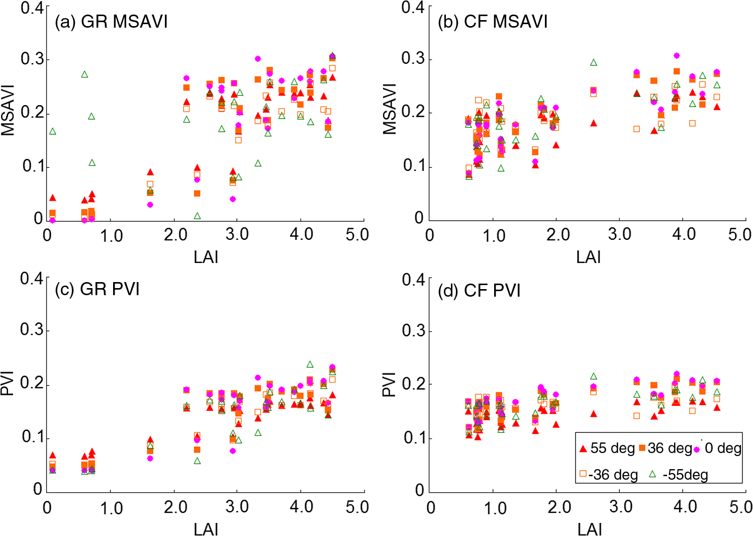 Both PVGT and P-VI indicate the differences of oblique/vertical and backward/forward observation angles. The least PVGT occurs at nadir (0 deg), demonstrating that the traditional “vertical” observation smooths the structural variations of vegetation types thanks to its monoangularly projected sampling. Though such smoothing to some degree results in better suitability to different vegetation types in LAI estimation, the information loss caused by the monoangle view is inevitable when we are interested in the differences of vegetation types. Thus, multiangular remote sensing compensates the loss by describing surface anisotropy of reflectance62 to better the estimation of true vegetation structures like LAI. The PVGTs from the backward series are greater than those from forward, and from more oblique angles greater than from less oblique, showing further the value of angular information in LAI estimation. This is mainly because of the less background potentially viewed in the oblique observation and more shadowing effects in the forward series. One of the general conclusions of off-nadir research is that it performs better than the mononadir in ecological monitoring;63 meanwhile, the land surface classification with backward data is better than with the forward.62–64 So, the anisotropy properties of vegetation reflectance have been increasingly investigated to improve the performance of VI in LAI estimation.65 The P-VIs from the backward series are also greater than from the forward. But different from PVGTs, P-VIs from less oblique angles are greater than from more oblique ones, and those from the nadir are the moderate. These results suggest that the nadir and forward observations do not perform differently when using various VIs in LAI estimation; on the contrary, choosing VIs from a backward less oblique angle () may benefit the estimation. Walter-Shea et al.66 also confirmed the advantage of a backward less oblique angle in the inversion of fraction of absorbed photosynthetically active radiation. Both PVGT and PANG are least for two traditional ratio-based VIs (NDVI and RVI), greatest PVGT for the multiband based (MCARI2), and greatest PANG for the soil adjusted (MSAVI and PVI). This implies the discrepancy of the applicability and discrimination of VIs to vegetation types and observation angles in LAI estimation. The two ratio-based indices perform most similarly in the estimation with the variations of either vegetation or angles, which is in accord with the findings by Kuusk.67 Similar to the applicability of nadir observation to different vegetation types, the cost of the “wider” suitability is the decreased discrimination of the vegetation and angle information of such VIs in the estimation. The MCARI2, the only VI involving three bands in our study, is most predictable to the variation of vegetation type, revealing that to account for the reflectance of the green band along with red and near-infrared bands in VI can improve its capability of describing vegetation structures.62 The PANGs are greatest for the two SAVIs, partly due to the fact that the soil-adjusted parameters were uniform in this study at all observation angles which contained different proportions of soil and the anisotropy of its reflectance within the field of view. The indistinctive adjustment of the soil effects possibly led to more a unstable LAI-VI response. We believe that integrating angular-oriented parameters to current SAVIs may potentially improve their performance in LAI estimation, which deserves further investigation. 3.4.Optimal Angle-Index Variables for Leaf Area Index EstimationTo sum up, the adaptability of the LAI-VI model is affected interactively by the variations in vegetation types, observation angles, and VIs. For each vegetation type, there is likely a suitable angle-index combination for LAI estimation. Using the method described in Sec. 2.4, multivariable linear regression models were established for each vegetation type. The results are shown in Table 3. Table 3Multivariable-based LAI-VI models for each vegetation type (LAI=c+b1×x1+b2×x2).
Except shrub, the determination coefficients () of the multivariable-based LAI-VI models for all vegetation types reach 0.7 to 0.9 and MREs range between 10% and 25%, showing anacceptable accuracy for most routine applications. The obvious less reliable model was established for shrub, which possibly resulted from its most sparse density (least LAI and VFC, Table 2). The background soil dominated the reflectance, leading to relatively poor LAI-VI relationships. Though the VIs selected in the model are adjusted to the soil effect, the adjustment requires further improvement according to the illuminate-viewing geometry. It is interesting to note the angle-index combinations selected in the linear models. Only two angles ( and 0 deg) and two indices (MSAVI and PVI) were selected in the modeling for all vegetation types, demonstrating the advantages of less oblique observation and soil-adjusted indices in multiangular LAI estimation. The nadir angle performs best for the two forest types with coniferous trees, suggesting the special potentials of the traditional “vertical” observation in LAI estimation for such forests. Rautiainen et al.58 found more significant anisotropy at 37 deg than at 57 deg of red and red-edge reflectances on coniferous forest. This seems not to provide valuable information in our study. One of the possible reasons is the difference of the structure, distribution, and optical properties of the studied vegetation. The backward less oblique angle () is the only one selected for the other three vegetation types. This is close to the findings of Goel and Qin,60 who argued that a less than 30 deg observation zenith angle was optimal for LAI estimation. The efficient viewing angle for the estimation is dependent upon both vegetation density and canopy anisotropy. The observation zenith angles suggested in the literature vary greatly, including ,66 ,68 ,62,69 and so on. Therefore, choosing a suitable observation angle is critical and requires more investigation in multiangular LAI estimation. The MSAVI was selected for all vegetations in the modeling, with the PVI for two dwarf vegetations (GR and SH). The advantages of less background soil effects and later saturation at high LAI regions9,21 were confirmed in our study. This indicated the importance of soil effects’ correction in multiangular LAI estimation, especially for dwarf or/and sparse vegetation communities. Increasing types of VIs were reported in literature62 using different angle-band combinations, pushing forward the exploitation of suitable VI for LAI estimation. The explicit suitability of VIs is difficult to concretely demonstrate; however, these results provide a reference to improve the estimation of vegetation structures using multiangular imagery. 4.ConclusionsThe predictability analysis of LAI-VI models was conducted in this study, using LAIs of five vegetation types: grass (GR), shrub (SH), coniferous forest (CF), coniferous and broad leaf forest (CB), and broad leaf forest (BF), and VIs from five observation angles of CHRIS/PROBA data. We calculated and compared three kinds of predictabilities, i.e., LAI-VI models to the variation of vegetation type (PVGT), observation angle (PANG), and VI (P-VI). Finally, we tested the chosen angle-index combination using the multivariable linear regression method. The following conclusions can be drawn:
AcknowledgmentsThis research was funded by the National Natural Science Foundation of China (No. 41071281), the Natural Science Foundation of Jiangsu Province (No. BK20131078), and the Qing Lan Project of Jiangsu Provincial Department of Education. Thanks Dr. Dongliang Li and Dr. Jianjun Cao from Nanjing Xiaozhuang University, for their help on field work and data analysis. We appreciate the careful improvement of English and many valuable suggestions from Kayla Stan and Dominica Harrison in Earth Observation Systems Laboratory, University of Alberta, Canada. We are very grateful to helpful comments and suggestions from anonymous reviewers, which improved the quality of this paper. ReferencesJ. M. Chen and T. A. Black,
“Defining leaf area index for non-flat leaves,”
Plant Cell Environ., 15
(4), 421
–429
(1992). http://dx.doi.org/10.1111/pce.1992.15.issue-4 0140-7791 Google Scholar
J. M. Chen et al.,
“Distributed hydrological model for mapping evapotranspiration using remote sensing inputs,”
J. Hydrol., 305
(1–4), 15
–39
(2005). http://dx.doi.org/10.1016/j.jhydrol.2004.08.029 JHYDA7 0022-1694 Google Scholar
Z. J. Gu et al.,
“Using multiple radiometric correction images to estimate leaf area index (LAI),”
Int. J. Remote Sens., 32
(24), 9441
–9454
(2011). http://dx.doi.org/10.1080/01431161.2011.562251 IJSEDK 0143-1161 Google Scholar
S. P. Serbin, D. E. Ahl and S. T. Gower,
“Spatial and temporal validation of the MODIS LAI and FPAR products across a boreal forest wildfire chronosequence,”
Remote Sens. Environ., 133
(1), 71
–84
(2013). http://dx.doi.org/10.1016/j.rse.2013.01.022 RSEEA7 0034-4257 Google Scholar
J. L. Zarate-Valdez et al.,
“Predictions of leaf area index in almonds by vegetation indexes,”
Comput. Electron. Agric., 85
(1), 24
–32
(2012). http://dx.doi.org/10.1016/j.compag.2012.03.009 CEAGE6 0168-1699 Google Scholar
B. B. He, X. W. Quan and M. F. Xing,
“Retrieval of leaf area index in alpine wetlands using a two-layer canopy reflectance model,”
Int. J. Appl. Earth Obs., 21
(1), 78
–91
(2013). http://dx.doi.org/10.1016/j.jag.2012.08.014 ITCJDP 0303-2434 Google Scholar
X. W. Quan et al.,
“Extended Fourier approach to improve the retrieved leaf area index (LAI) in a time series from an alpine wetland,”
Remote Sens., 6
(2), 1171
–1190
(2014). http://dx.doi.org/10.3390/rs6021171 2072-4292 Google Scholar
R. Colombo et al.,
“Retrieval of leaf area index in different vegetation types using high resolution satellite data,”
Remote Sens. Environ., 86
(1), 120
–131
(2003). http://dx.doi.org/10.1016/S0034-4257(03)00094-4 RSEEA7 0034-4257 Google Scholar
J. D. Wu, D. Wang and M. E. Bauer,
“Assessing broadband vegetation indices and QuickBird data in estimating leaf area index of corn and potato canopies,”
Field Crops Res., 102
(1), 33
–42
(2007). http://dx.doi.org/10.1016/j.fcr.2007.01.003 FCREDZ 0378-4290 Google Scholar
N. Gobron, B. Pinty and M. M. Verstraete,
“Theoretical limits to the estimation of the leaf area index on the basis of visible and near-infrared remote sensing data,”
IEEE Trans. Geosci. Remote Sens., 35
(6), 1438
–1445
(1997). http://dx.doi.org/10.1109/36.649798 IGRSD2 0196-2892 Google Scholar
I. Ozdemir,
“Linear transformation to minimize the effects of variability in understory to estimate percent tree canopy cover using RapidEye data,”
Geosci. Remote Sens., 51
(3), 288
–300
(2014). http://dx.doi.org/10.1080/15481603.2014.912876 IGRSBY 1545-598X Google Scholar
J. M. B. Carreiras, J. M. C. Pereira and J. S. Pereira,
“Estimation of tree canopy cover in evergreen oak woodlands using remote sensing,”
For. Ecol. Manage., 223 45
–53
(2006). http://dx.doi.org/10.1016/j.foreco.2005.10.056 FECMDW 0378-1127 Google Scholar
G. Asrar, E. T. Kanemasu and M. Yoshida,
“Estimates of leaf area index from spectral reflectance of wheat under different cultural practices and solar angle,”
Remote Sens. Environ., 17
(1), 1
–11
(1985). http://dx.doi.org/10.1016/0034-4257(85)90108-7 RSEEA7 0034-4257 Google Scholar
R. G. Best and J. C. Harlan,
“Spectral estimation of green leaf area index of oats,”
Remote Sens. Environ., 17
(1), 27
–36
(1985). http://dx.doi.org/10.1016/0034-4257(85)90110-5 RSEEA7 0034-4257 Google Scholar
B. R. Gardner and B. L. Blad,
“Evaluation of spectral reflectance models to estimate corn leaf area while minimizing the influence of soil background effects,”
Remote Sens. Environ., 20
(2), 183
–193
(1986). http://dx.doi.org/10.1016/0034-4257(86)90022-2 RSEEA7 0034-4257 Google Scholar
C. L. Wiegand et al.,
“Vegetation indices in crop assessments,”
Remote Sens. Environ., 35
(2–3), 105
–119
(1991). http://dx.doi.org/10.1016/0034-4257(91)90004-P RSEEA7 0034-4257 Google Scholar
R. L. Weiser et al.,
“Assessing grassland biophysical characteristics from spectral measurements,”
Remote Sens. Environ., 20
(2), 141
–152
(1986). http://dx.doi.org/10.1016/0034-4257(86)90019-2 RSEEA7 0034-4257 Google Scholar
B. E. Law and R. H. Waring,
“Remote sensing of leaf area index and radiation intercepted by understory vegetation,”
Ecol. Appl., 4
(2), 272
–279
(1994). http://dx.doi.org/10.2307/1941933 ECAPE7 1051-0761 Google Scholar
M. A. Spanner, L. L. Pierce and S. W. Running,
“The seasonality of AVHRR data of temperate coniferous forests: relationship with leaf area index,”
Remote Sens. Environ., 33
(2), 97
–112
(1990). http://dx.doi.org/10.1016/0034-4257(90)90036-L RSEEA7 0034-4257 Google Scholar
H. L. Fang, S. S. Wei and C.Y. Jiang,
“Klaus Scipal theoretical uncertainty analysis of global MODIS, CYCLOPES and GLOBCARBON LAI products using a triple collocation method,”
Remote Sens. Environ., 124
(1), 610
–621
(2012). http://dx.doi.org/10.1016/j.rse.2012.06.013 RSEEA7 0034-4257 Google Scholar
D. Haboudane et al.,
“Hyperspectral vegetation indices and novel algorithms for predicting green LAI of crop canopies: modeling and validation in the context of precision agriculture,”
Remote Sens. Environ., 90
(3), 337
–352
(2004). http://dx.doi.org/10.1016/j.rse.2003.12.013 RSEEA7 0034-4257 Google Scholar
A. Viña et al.,
“Comparison of different vegetation indices for the remote assessment of green leaf area index of crops,”
Remote Sens. Environ., 115
(12), 3468
–3478
(2011). http://dx.doi.org/10.1016/j.rse.2011.08.010 RSEEA7 0034-4257 Google Scholar
Z. J. Gu et al.,
“Applicability of spectral and spatial information from IKONOS_2 imagery in retrieving leaf area index of forests in the urban area of Nanjing, China,”
J. Appl. Remote Sens., 6 063556
(2012). http://dx.doi.org/10.1117/1.JRS.6.063556 1931-3195 Google Scholar
R. B. Pollock and E. T. Kanemasu,
“Estimating leaf-area index of wheat with LANDSAT data,”
Remote Sens. Environ., 8
(4), 307
–312
(1979). http://dx.doi.org/10.1016/0034-4257(79)90030-0 RSEEA7 0034-4257 Google Scholar
P. Boissard et al.,
“Application of SPOT data to wheat yield estimation,”
Adv. Space Res., 9
(1), 143
–154
(1989). http://dx.doi.org/10.1016/0273-1177(89)90479-1 ASRSDW 0273-1177 Google Scholar
A. R. Huete et al.,
“Normalization of multidirectional red and NIR reflectances with the SAVI,”
Remote Sens. Environ., 41
(2–3), 143
–154
(1992). http://dx.doi.org/10.1016/0034-4257(92)90074-T RSEEA7 0034-4257 Google Scholar
C. B. Schaaf et al.,
“First operational BRDF, albedo nadir reflectance products from MODIS,”
Remote Sens. Environ., 83
(1–2), 135
–148
(2002). http://dx.doi.org/10.1016/S0034-4257(02)00091-3 RSEEA7 0034-4257 Google Scholar
D. J. Diner et al.,
“New directions in earth observing: scientific applications of mutiangle remote sensing,”
Bull. Am. Meteorol. Soc., 80
(11), 2209
–2228
(1999). http://dx.doi.org/10.1175/1520-0477(1999)080<2209:NDIEOS>2.0.CO;2 BAMIAT 0003-0007 Google Scholar
Y. J. Yao et al.,
“LAI retrieval and uncertainty evaluations for typical row-planted crops at different growth stages,”
Remote Sens. Environ., 112
(1), 94
–106
(2008). http://dx.doi.org/10.1016/j.rse.2006.09.037 RSEEA7 0034-4257 Google Scholar
R. D. Jackson et al.,
“Bidirectional measurements of surface reflectance for view angle corrections of oblique imagery,”
Remote Sens. Environ., 32
(2–3), 189
–202
(1990). http://dx.doi.org/10.1016/0034-4257(90)90017-G RSEEA7 0034-4257 Google Scholar
F. Gemmell and A. J. McDonald,
“View zenith angle effects on the forest information content of tree spectral indices,”
Remote Sens. Environ., 72
(2), 139
–158
(2000). http://dx.doi.org/10.1016/S0034-4257(99)00086-3 RSEEA7 0034-4257 Google Scholar
J. Verrelst et al.,
“Angular sensitivity analysis of vegetation indices derived from CHRIS/PROBA data,”
Remote Sens. Environ., 112
(5), 2341
–2353
(2008). http://dx.doi.org/10.1016/j.rse.2007.11.001 RSEEA7 0034-4257 Google Scholar
A. Bannari et al.,
“A review of vegetation indices,”
Remote Sens. Rev., 13
(1–2), 95
–120
(1995). http://dx.doi.org/10.1080/02757259509532298 RSRVEP 0275-7257 Google Scholar
S. Moulin and M. Guerif,
“Impacts of model parameter uncertainties on crop reflectance estimates: a regional case study on wheat,”
Int. J. Remote Sens., 20
(1), 213
–218
(1999). http://dx.doi.org/10.1080/014311699213730 IJSEDK 0143-1161 Google Scholar
J. W. Rouse and R. H. Hass,
“Monitoring vegetation systems in the Great Plains with ERTS,”
in Proc. Third ERTS Symp.,
309
–317
(1974). Google Scholar
C. J. Tucker,
“Red and photographic infrared linear combinations for monitoring vegetation,”
Remote Sens. Environ., 8
(2), 127
–150
(1979). http://dx.doi.org/10.1016/0034-4257(79)90013-0 RSEEA7 0034-4257 Google Scholar
F. Baret and G. Guyot,
“Potentials and limits of vegetation indices for LAI and APAR assessment,”
Remote Sens. Environ., 35
(2–3), 161
–173
(1991). http://dx.doi.org/10.1016/0034-4257(91)90009-U RSEEA7 0034-4257 Google Scholar
A. J. Richardson and C. L. Wiegand,
“Distinguishing vegetation from soil background information,”
Photogramm. Eng. Remote Sens., 43
(12), 1541
–1552
(1977). PGMEA9 0099-1112 Google Scholar
A. R. Huete,
“A soil adjusted vegetation index (SAVI),”
Remote Sens. Environ., 25
(3), 295
–309
(1988). http://dx.doi.org/10.1016/0034-4257(88)90106-X RSEEA7 0034-4257 Google Scholar
Ts. Purevdorj et al.,
“Relationships between percent vegetation cover and vegetation indices,”
Int. J. Remote Sens., 19
(18), 3519
–3535
(1998). http://dx.doi.org/10.1080/014311698213795 IJSEDK 0143-1161 Google Scholar
F. Baret, G. Guyot and D. J. Major,
“TSAVI: a vegetation index which minimizes soil brightness effects on LAI and APAR estimation,”
in Proc. 12th Canadian Symp. Remote Sensing IGARSS’89,
1355
–1358
(1989). Google Scholar
J. Qi et al.,
“A modified soil adjusted vegetation index,”
Remote Sens. Environ., 48
(2), 119
–126
(1994). http://dx.doi.org/10.1016/0034-4257(94)90134-1 RSEEA7 0034-4257 Google Scholar
Y. J. Kaufman and D. Tanré,
“Atmospherically resistant vegetation index (ARVI) for EOS-MODIS,”
IEEE Trans. Geosci. Remote Sens., 30
(2), 261
–270
(1992). http://dx.doi.org/10.1109/36.134076 IGRSD2 0196-2892 Google Scholar
A. R. Huete et al.,
“A comparison of vegetation indices over a global set of TM images for EOS-MODIS,”
Remote Sens. Environ., 59
(3), 440
–451
(1997). http://dx.doi.org/10.1016/S0034-4257(96)00112-5 RSEEA7 0034-4257 Google Scholar
S. T. Brantley, J. C. Zinnert and D. R. Young,
“Application of hyperspectral vegetation indices to detect variations in high leaf area index temperate shrub thicket canopies,”
Remote Sens. Environ., 115
(2), 514
–523
(2011). http://dx.doi.org/10.1016/j.rse.2010.09.020 RSEEA7 0034-4257 Google Scholar
C. Mike, CHRIS Data Format, 37
(2008). Google Scholar
J. Cernicharo, A. Verger and F. Camacho,
“Empirical and physical estimation of canopy water content from CHRIS/PROBA data,”
Remote Sens., 5
(10), 5265
–5284
(2013). http://dx.doi.org/10.3390/rs5105265 2072-4292 Google Scholar
S. Ringrose et al.,
“Vegetation cover trends along the Botswana Kalahari transect,”
J. Arid Environ., 54
(2), 297
–317
(2003). http://dx.doi.org/10.1006/jare.2002.1092 JAENDR Google Scholar
Z. J. Gu et al.,
“A model for estimating total forest coverage with ground-based digital photography,”
Pedosphere, 20
(3), 318
–325
(2010). http://dx.doi.org/10.1016/S1002-0160(10)60020-3 PDOSEA Google Scholar
L. Guanter, L. Alonso and J. Moreno,
“Atmospheric correction of CHRIS/PROBA data acquired in the SPARC campaign,”
in Proc. 2nd CHRIS/PROBA Workshop,
(2004). Google Scholar
C. F. Jordan,
“Derivation of leaf area index from quality of light on the forest floor,”
Ecology, 50
(4), 663
–666
(1969). http://dx.doi.org/10.2307/1936256 ECOLAR 0012-9658 Google Scholar
D. Haboudane et al.,
“Hyperspectral vegetation indices and novel algorithms for predicting green LAI of crop canopies: modeling and validation in the context of precision agriculture,”
Remote Sens. Environ., 90 337
–352
(2004). http://dx.doi.org/10.1016/j.rse.2003.12.013 RSEEA7 0034-4257 Google Scholar
C. Y. Wu et al.,
“Predicting leaf area index in wheat using angular vegetation indices derived from in situ canopy measurements,”
Can. J. Remote Sens., 36
(4), 301
–312
(2014). http://dx.doi.org/10.5589/m10-050 CJRSDP 0703-8992 Google Scholar
A. Nguy-Robertson et al.,
“Green leaf area index estimation in maize and soybean: combining vegetation indices to achieve maximal sensitivity,”
Agron. J., 104
(5), 1336
–1347
(2012). http://dx.doi.org/10.2134/agronj2012.0065 AGJOAT 0002-1962 Google Scholar
J. C. Jiménez-Muñoz et al.,
“Comparison between fractional vegetation cover retrievals from vegetation indices and spectral mixture analysis case study of PROBA/CHRIS data over an agricultural area,”
Sensors, 9
(2), 768
–793
(2009). http://dx.doi.org/10.3390/s90200768 SNSRES 0746-9462 Google Scholar
J. P. Gastellu-Etchegorry et al.,
“Modeling BRF and radiation regime of boreal and tropical forests: I. BRF,”
Remote Sens. Environ., 68
(3), 281
–316
(1999). http://dx.doi.org/10.1016/S0034-4257(98)00119-9 RSEEA7 0034-4257 Google Scholar
Z. J. Gu et al.,
“Assessing factors influencing vegetation coverage calculation with remote sensing imagery,”
Int. J. Remote Sens., 30
(10), 2479
–2489
(2009). http://dx.doi.org/10.1080/01431160802552736 IJSEDK 0143-1161 Google Scholar
M. Rautiainen et al.,
“Multi-angular reflectance properties of a hemiboreal forest: an analysis using CHRIS PROBA data,”
Remote Sens. Environ., 112
(5), 2627
–2642
(2008). http://dx.doi.org/10.1016/j.rse.2007.12.005 RSEEA7 0034-4257 Google Scholar
J. M. Chen et al.,
“Multi-angular optical remote sensing for assessing vegetation structure and carbon absorption,”
Remote Sens. Environ., 84
(4), 516
–525
(2003). http://dx.doi.org/10.1016/S0034-4257(02)00150-5 RSEEA7 0034-4257 Google Scholar
N. S. Goel and W. H. Qin,
“Influences of canopy architecture on relationships between various vegetation indices and LAI and Fpar A computer simulation,”
Remote Sens. Rev., 10
(4), 309
–347
(1994). http://dx.doi.org/10.1080/02757259409532252 RSRVEP 0275-7257 Google Scholar
K. J. Ranson et al.,
“Sun-view angle effects on reflectance factors of corn canopies,”
Remote Sens. Environ., 18
(2), 147
–161
(1985). http://dx.doi.org/10.1016/0034-4257(85)90045-8 RSEEA7 0034-4257 Google Scholar
S. Stagakis et al.,
“Monitoring canopy biophysical and biochemical parameters in ecosystem scale using satellite hyperspectral imagery: an application on a Phlomis fruticosa Mediterranean ecosystem using multiangular CHRIS/PROBA observations,”
Remote Sens. Environ., 114
(5), 977
–994
(2010). http://dx.doi.org/10.1016/j.rse.2009.12.006 RSEEA7 0034-4257 Google Scholar
L. S. Galvão et al.,
“View angle effects on the discrimination of soybean varieties and on the relationships between vegetation indices and yield using off-nadir Hyperion data,”
Remote Sens. Environ., 113
(4), 846
–856
(2009). http://dx.doi.org/10.1016/j.rse.2008.12.010 RSEEA7 0034-4257 Google Scholar
V. Liesenberg, L. S. Galvão and F. J. Ponzoni,
“Variations in reflectance with seasonality and viewing geometry: implications for classification of Brazilian savanna physiognomies with MISR/Terra data,”
Remote Sens. Environ., 107
(1–2), 276
–286
(2007). http://dx.doi.org/10.1016/j.rse.2006.03.018 RSEEA7 0034-4257 Google Scholar
A. A. Gitelson, Y. Peng and K. F. Huemmrich,
“Relationship between fraction of radiation absorbed by photosynthesizing maize and soybean canopies and NDVI from remotely sensed data taken at close range and from MODIS 250 m resolution data,”
Remote Sens. Environ., 147 108
–120
(2014). http://dx.doi.org/10.1016/j.rse.2014.02.014 RSEEA7 0034-4257 Google Scholar
E. A. Walter-Shea et al.,
“Relations between directional spectral vegetation indices and leaf area and absorbed radiation in alfalfa,”
Remote Sens. Environ., 61
(1), 162
–177
(1997). http://dx.doi.org/10.1016/S0034-4257(96)00250-7 RSEEA7 0034-4257 Google Scholar
A. Kuusk,
“The angular distribution of reflectance and vegetation indices in barley and clover canopies,”
Remote Sens. Environ., 37
(2), 143
–151
(1991). http://dx.doi.org/10.1016/0034-4257(91)90025-2 RSEEA7 0034-4257 Google Scholar
G. G. Gutman,
“Vegetation indices from AVHRR: an update and future prospects,”
Remote Sens. Environ., 35
(2–3), 121
–136
(1991). http://dx.doi.org/10.1016/0034-4257(91)90005-Q RSEEA7 0034-4257 Google Scholar
S. Huber et al.,
“The potential of spectrodirectional CHRIS/PROBA data for biochemistry estimation,”
in Proc. Envisat Symposium 2007,
(2007). Google Scholar
BiographyZhujun Gu is currently a visiting scholar at the Earth Observation Systems Laboratory, Department of Earth and Atmospheric Sciences, University of Alberta, Canada. He received his BSc degree in 1993 and his MSc degree in 2005 from the Department of Geography at Nanjing Normal University, China, and his PhD degree in 2008 from the State Key Laboratory of Soil and Sustainable Agriculture, Institute of Soil Science, Chinese Academy of Sciences, China. He is an associate professor at the School of Environmental Science, Nanjing Xiaozhuang University, China. His research interests include remote sensing of vegetation structures and soil and water conservation. G. Arturo Sanchez-Azofeifa is a full professor at the Department of Earth and Atmospheric Sciences at the University of Alberta. His research focuses on characterizing the growth dynamics of tropical forests using LiDAR, wireless sensor networks, and hyperspectral remote sensing. His research also involves the study of theoretical linkages between remote sensing (multispectral and hyperspectral) and the spectrotemporal dynamics of leaf area index, primary productivity, and photosynthetic active radiation in tropical dry forests of the Americas. Jilu Feng received his MS degree in cartography and remote sensing from Peking University, China, and his PhD degree in earth and atmospheric sciences from the University of Alberta, Canada, in 1991 and 2002, respectively. His research interests have included the use of hyperspectral data for mineral mapping and the development of new algorithms for target detection. Current research projects include automatic core logging from hyperspectral devices and quick characterization of oil sand from reflectance spectroscopy. Sen Cao received his BS degree in geographical information science from Sun Yat-sen University, China, in 2010. He is currently working toward his PhD degree at Beijing Normal University, Beijing, China, and is now a visiting student at the University of Alberta, Canada. His research interests include remote sensing image registration, environmental mapping, and productivity estimation. |
||||||||||||||||||||||||||||||||||||||||||||||||||||||||||||||||||||||||||||||||||||||||||||||||||||||||||||||||||||||||||||||||||||||||||||||||||


