1.

Introduction

Biomass, in ecology, is the mass of living organisms in a given area or ecosystem at a given time.¹ Here, as in most of the literature on the carbon cycle and remote sensing, biomass refers to the total dry weight of organic aboveground plant matter in a unit surface area. Wetlands, an important component of terrestrial ecosystems, play a key role in global climate change because one of their components, wetland vegetation, is the main source of the carbon in the atmosphere.² Wetland vegetation biomass is a key indicator for evaluating the carbon sequestration capacity of wetlands. Biomass governs the potential amount of carbon that could be released into the atmosphere because of deforestation, and regional biomass changes have been associated with important outcomes in ecosystem functional characteristics and climate change.³ Therefore, biomass estimation of the wetland vegetation plays a key role in the understanding of dynamic changes of wetland ecosystems. Generally, conventional field methods of biomass estimation are time consuming and labor intensive and cannot provide details on the spatial distribution of a biomass. The advantages of remote sensing data, especially synthetic aperture radar (SAR) data, are that it can be collected repeatedly and processed conveniently, making it an efficient data source for large-area biomass retrieval, especially in areas of difficult access. Lu pointed out that remote sensing data have been the main data source for biomass estimation and are attracting increased attention from scientific researchers.³

Optical data can be used to extract spectral information in the form of the vegetation index, which is related to the biomass and can be used to retrieve biomass by application of a regression model.^4,5 However, in areas of dense vegetation, saturation in optical bands influences the precision in this biomass inversion.⁵ Because SAR is able to penetrate vegetation and to operate at all times and in all types of weather and because it saturates only at very high levels of energy, it can be used to retrieve vegetation biophysical parameters (VBPs).⁶

Many studies have shown that SAR can be used to retrieve vegetation biomass. Henderson and Lewis reviewed the recent research from five major remote sensing journals, spanning the years 1965 to 2007, and found that the C-band is necessary for herbaceous wetland detection. HH polarization is preferable to VV, but cross-polarized data seem to contribute more than was thought earlier in some cases.⁷ Kasischke et al. concluded that imaging radar was suitable for ecological applications, especially the delineation of wetland inundation, vegetative cover, and the measurement of aboveground plant biomass.⁸ Lu reviewed radar data for biomass estimation and discussed the common saturation problem in radar data.³ Baghdadi et al. have evaluated the use of C-band polarimetric SAR (PolSAR) data for wetland mapping,⁹ and the results have shown that the HH and cross-polarizations are better than VV polarization and the cross-polarization data can provide the best separation. Srivastava et al. explored the potential of multiparametric (multi-incidence angle, multipolarized, temporal, high-resolution, and multifrequency) SAR data in wetland inventories and suggested that SAR data have a number of unique features that can be exploited in the assessment, monitoring, and management of a wetland ecosystem. Srivastava et al. also addressed the interaction of radar signals (frequency, incidence angle, and polarization) with various components of a wetland ecosystem (moisture content of vegetation or soil, surface roughness, structure of the vegetation, textural properties of the target, orientation of the target, etc.).⁶

Liao et al. and Shen et al. have retrieved the Poyang Lake wetland vegetation biomass using ENVISAT ASAR data with an artificial neural network (ANN).^10–12 Shen et al. and Yang et al. found that the fresh biomass of rice has a good relation with the backscatter coefficient of ENVISAT ASAR data with HH and HV polarizations.^13,14 Because ASAR data are nonpolarimetric, the polarized difference and polarization ratio were used to improve the precision of the inversion procedure.¹¹ To optimize livestock management in a water-saturated Andean wetland, Moreau and Toan used ERS SAR data to retrieve spatio-temporal information on the biomass of totora reeds and bofedal, which are a critical foraging resource for smallholders.¹⁵ The radar backscattering coefficient (${\sigma }^0$ measured in dB), measured by ERS, was found to be sensitive to both the humid and the dry biomass of totora reeds and bofedal grasslands. The sensitivity of the signal-to-biomass variation is high for dry biomass, less than $1\mathrm{kg}/{\mathrm{m}}^2$ for totora, and less than $2\mathrm{kg}/{\mathrm{m}}^2$ for bofedal.¹⁵ Yang et al. used relational models based on the analysis of the correlation between backscatter coefficients and field measurements to retrieve rice growth parameters from ASAR images.¹⁴

Polarimetric information can significantly improve wetland vegetation characterization for wetland mapping.^16,17 Slatton et al. modeled wetland vegetation by using airborne PolSAR in herbaceous coastal wetlands in the C-, L-, and P-bands and showed that PolSAR has the potential for mapping coastal herbaceous wetlands.¹⁸ The short-wavelength SAR (X- and C-bands) interacts with the upper part of the crop canopy, thus offering the potential for retrieving crop biophysical parameters.¹⁹ The use of polarimetric RADARSAT-2 data has been investigated for operational mapping and for monitoring Canadian wetlands^16,20 and the Poyang Lake wetland.^21,22 Inoue et al. found that the backscatters from a polarimetric scatterometer are sensitive to rice biomass and have some connection with the angular distribution and size of the plant elements (leaves, stems, and heads).²³ Target scattering decomposition has become a popular method for extracting the geophysical parameters of a natural target from PolSAR data,²⁴ which can lead to unique parameters that optimize wetland classification.^20–22 Li et al. proposed a new inversion method for vegetation parameters based on the Freeman polarization decomposition.²⁵

Retrieving wetland vegetation biomass from SAR data has often been carried out by implementation of linear and nonlinear multiple regressions. However, the performance is influenced by the highly complex nonlinear relation between vegetation biomass and the SAR backscatter. An alternative approach, based on ANN algorithms, which are becoming commonly available and readily usable, has been devised to retrieve environmental parameters from SAR data. ANNs are composed of many nonlinear computational elements such as neurons, operating in parallel and linked with each other through connections characterized by multiplying factors. This structure makes ANNs inherently suitable for addressing nonlinear problems.²⁶ The use of these algorithms in remote sensing has often been found effective because they can simultaneously handle nonlinear mapping of a multidimensional input space onto the output space and also cope with complex statistical behavior. Jin and Liu used the experimental data obtained from active/passive microwave remote sensing and from ground-truth measurements to train the ANN to retrieve biomass parameters.²⁷ The ANN model was first trained by using wheat canopy data from 1988, and was then used to retrieve biomass parameters of wheat canopy during growth in l989, which was compared with the ground-truth data. Frate and Wang applied an electromagnetic model and neural network algorithms to retrieve the biomass for sunflower fields using radar backscattering data. The electromagnetic model was used to generate the scattering coefficients for training and testing the network. The inversion results showed that the neural network was capable of performing the retrieval with good accuracy. By optimizing the structural complexity of the net, these researchers obtained a better inversion result.²⁶ Frate and Wang used ANN to retrieve forest biomass from multifrequency (L- and P-bands), multipolarization (HH, VV, and HV) backscattering, after the training and pruning procedures had been made to the net, and compared the ANN retrieval accuracy with that yielded by linear and nonlinear regressions and by a model-based technique.²⁸

In this study, polarimetric RADARSAT-2 data were used to retrieve vegetation biomass in the Poyang Lake wetland. First, the backscatter from vegetation was simulated on the basis of the canopy backscatter model. Then, the Freeman polarimetric decomposition components and HH, VV, and HV polarization backscatters from RADARSAT-2 data were used as the inputs to an ANN to retrieve the VBPs. Finally, the retrieved VBPs and Freeman polarimetric decomposition components were used as the inputs to another ANN to retrieve the biomass.

2.

Study Area and Data

2.1.

Study Area

The test site is located in the Poyang Lake wetland (inland lake wetland), Jiangxi Province, China in the lower Yangtze River Basin. The latitude and longitude are 28°22′–29°15′ N and 115°47′–116°45′ E (Fig. 1). The climate is characterized as a subtropical, humid, monsoon climate with a 1620 mm mean annual precipitation, and an annual average temperature of approximately 17°C. In summer, Poyang Lake is the largest freshwater body in China. By the end of the rainy season, the lake can extend up to $3500{\mathrm{km}}^2$ in area, but during the dry season, it may shrink to less than $1000{\mathrm{km}}^2$ and become a system of sublakes interspersed with mudflats, sediment beds, and vegetation. The variation in the water level of Poyang Lake during the year is very large. In 2007, the absolute fluctuation of the water level was up to 8.37 m. The area of the lake greatly varies with the fluctuation of its water level. The water level rises during the flood season, and the water surface suddenly expands. The water level drops during the dry season, and the lakebed appears and only a few wandering watercourses remain. In summary, the test site has dry and wet seasons. In the dry season (November to April), the wetland vegetation is above the water. It starts to rapidly grow from early spring, with the biomass reaching its highest level in April.²⁹ In the wet season (June to September), the wetland vegetation is flooded and hardly grows.

Fig. 1

Spatial location and extent of the study area of Poyang Lake, Jiangxi Province, People’s Republic of China. The red polygon shows the extent of Poyang Lake wetland, the black polygon shows the extent of the RADARSAT-2 imagery acquired on April 8, 2011, and the green polygon shows the Nanjishan National Nature Reserve. (a) The Pauli decomposition image, (b) and (c) Landsat ETM+ acquired on February 4, 2003.

The predominant vegetation in Poyang Lake is carex and reed [Fig. 4(a)], which together cover more than 90% of the area.^29,30 The height, water content, and plant density of the vegetation vary with the different hydrological stages from April to November. In April, the carex rapidly grows with green leaves of approximately 30 to $70{\mathrm{cm}}^2$. In July, the plants are submerged in the water, and in November they turn yellow and the water content of the plants decreases.

The study area (the RADARSAT-2’s coverage) is mainly located in the southwest part of Poyang Lake wetland known as the Nanjishan National Nature Reserve (the green polygon in Fig. 1), covering an area of $\mathrm{33,300}{\mathrm{hm}}^2$. The land cover of the Nanjishan Wetland Nature Reserve consists of a profundal zone, swamp, marsh, sandy land, and grassland, where the predominant vegetation is also carex and reed.³¹

2.3.

Field Survey

Because ground-truth data collection in a wetland is difficult to access, time consuming, and tedious,³² a quasisynchronous field survey was conducted in Poyang Lake wetland from April 7, 2011 to April 10, 2011. Within the area covered by the RADARSAT-2 imagery, 2 to 3 sample points ($0.5\times 0.5{\mathrm{m}}^2$ or $1\times 1{\mathrm{m}}^2$) were randomly selected for each sample area, and 54 sample points within different sample areas (with intersite spacing $>50\mathrm{m}$, 10 times the pixel size) were collected (Fig. 1).³² At each sample point, the fresh biomass, total height, stem height, stem density, stem diameter, leaf length, leaf width, leaf thickness, leaf number per plant, and the longitude and latitude of the sample point were recorded. After the grass was harvested, it was immediately weighed to determine the fresh biomass. The grass was then dried in an oven for 30 min at 120°C, and then dried to constant weight at 80°C to get the dry biomass and the moisture content.³³ Because of the severe drought in April 2011,³⁴ the dry biomass was a little lighter than the sample weight in the survey conducted from March 29 to April 3, 2007.¹¹

According to ground-truth data, the dry biomass was well correlated with the vegetation height, stem-layer height, leaf length, leaf width, and stem diameter [Figs. 2(a) to 2(e)], but not so well with leaf number density [Fig. 2(f)]. The dry biomass negatively correlated with the vegetation moisture content [Fig. 2(g)]. Therefore, these parameters (the vegetation height, stem-layer height, leaf length, leaf width, stem diameter, and vegetation moisture) can be used to retrieve the dry aboveground biomass of the vegetation (The following discussion will be based on the dry aboveground biomass).

Fig. 2

Relation between the dry biomass and various vegetation biophysical parameters, (a) for vegetation height, (b) for stem layer height, (c) for leaf length, (d) for leaf width, (e) for stem diameter, (f) for leaf number density, and (g) for vegetation moisture content.

3.

Method

3.1.

RADARSAT-2 Data Processing

First, the RADARSAT-2 image was calibrated to the Sinclair matrix by use of the sigma look-up table.³⁵ Next, the backscatter coefficients (${\sigma }^0$) for HH, HV/VH, and VV polarizations, as well as the coherency elements, $T3$, were calculated. To reduce the speckle, the data were filtered through the Lee refined filter³⁶ with a window size of $3\times 3$. The Freeman polarimetric decomposition assumes that the covariance matrix of the backscattering data can be decomposed into three covariance matrices, corresponding to scattering mechanisms of the following types: direct surface (odd-bounce), dihedral-type (double and even-bounce), and a random volume.³⁷ Thus, the Freeman three-component decomposition method was used to extract the components representing the volume, double-bounce, and surface scattering (Fig. 3).^37,38 From the top left of Fig. 3, it can be seen that the predominant backscattering for wetland vegetation is volume scattering (Region A). However, at the lakeshore (Region B), the vegetation displays as red or yellow because of the high double-bounce scattering between the sparse vegetation and the ground.³⁹ The predominant scattering for the mudbank (Region C) near the open water is surface scattering. Surface scattering is dominant for some of the water (Region D) because of the flotsam, but in some ponds (Region E), surface scattering (specular reflection) is dominant and results in the weak backscatter.

Fig. 3

Composite map of Freeman polarimetric decomposition.

All the data (the ${\sigma }^0$ under HH, HV/VH, VV polarizations; the three components under Freeman decomposition) were projected to the same projection, which could be easily used to extract the sample points’ backscatter coefficients and the polarimetric decomposition components by use of their coordinates. To determine the vegetation extent, the unsupervised H-A-alpha-Wishart classification method^40,41 was used to classify the extent of the water body and lakeshore. The classification result can be derived from Fig. 8, which divided the land cover into four types: grassland with different vegetation biomass level, water, lakeshore, and others (NULL in Fig. 8).

3.2.

Backscatter Simulation

The canopy backscatter model used in this work⁴² was modified on the basis of Karam’s forest canopy scattering model,⁴³ which fits the scattering by rice at different growth stages. The model was used to simulate the wetland vegetation’s backscatter. This simulation could be done because the model has a similar structure to rice but has a greater density (Fig. 4). Zhang used this modified model to retrieve the rice parameters.⁴⁴ Here, the backscatter model was used to analyze the radar backscatter sensitivity to the wetland VBPs.

Fig. 4

(a) Poyang Lake wetland vegetation and (b) the diagram used in the backscatter model.

Because of the high vegetation coverage, it was assumed that the only vegetation within the study area was carex. There were three layers: (1) the leaf layer, (2) the trunk layer, and (3) the ground. There was no ear layer. Thus, the total backscatter can be expressed as

Eq. (1)

$${\sigma }_{\text{total}}={\sigma }_{\text{leaf}}+{\sigma }_{\text{leaf}\text{-}\text{ground}}+{\sigma }_{\text{stem}}+{\sigma }_{\text{stem}\text{-}\text{ground}}+{\sigma }_{\text{ground}},$$

where ${\sigma }_{\text{total}}$ is the total backscatter, ${\sigma }_{\text{leaf}}$ and ${\sigma }_{\text{stem}}$ are the volume backscatters from leaf and stem, ${\sigma }_{\text{leaf}\text{-}\text{ground}}$ and ${\sigma }_{\text{stem}\text{-}\text{ground}}$ are the double-bounce backscatters introduced by the interaction between the leaf, stem, and the ground, and ${\sigma }_{\text{ground}}$ is the direct backscatter from the ground. In this model, the Debye−Cole model was used to calculate the dielectric constant of the vegetation canopy.⁴⁵ The inputs to the backscatter model are listed in Table 2.

Table 2

Statistics for the wetland vegetation parameters (inputs for the backscatter model).

Number	Parameter	Mean	Max	Min	Std. Dev.
1	Leaf half length (cm)	13.32	20.42	7.58	2.78
2	Leaf half width (mm)	2.05	2.75	1.33	0.28
3	Leaf half depth (thickness, mm)	0.11	0.20	0.07	0.02
4	Leaf number density ($\mathrm{N}/{\mathrm{m}}^2$)	11,801	18,928	4536	3688
5	Vegetation moisture content (%)	79.51	83.91	75.16	1.82
6	Vegetation height (cm)	48.95	67.67	37.67	6.01
7	Stem-layer height (cm)	15.39	29.17	9.8	4.08
8	Stem diameter (mm)	2.22	2.88	1.41	0.33
9	Stem density ($\mathrm{N}/{\mathrm{m}}^2$)	2096	3548	648	669
10	Wet aboveground biomass ($\mathrm{g}/{\mathrm{m}}^2$)	1650.1	2363.6	870.3	368.5
11	Dry aboveground biomass ($\mathrm{g}/{\mathrm{m}}^2$)	348.8	571.2	181.0	80.97

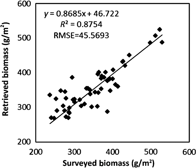
Because of the wetland environment with high soil moisture (nearly saturated), the ground could be considered flooded in most cases. The flooded ground results in weak direct backscatter from the ground (water) because of specular reflection, but the ground can still contribute to the double-bounce between it and the leaf and stem, whereas the nonflooded ground can also contribute to the two-way attenuation (SAR signal coming to ground and then going back to the sensor through the vegetation).^46,47 In addition, because of the same growth stage when the field survey was conducted, the vegetation moisture scatters closely around 80%, as did the vegetation moisture from the former field surveys.¹¹ However, the different canopy height and density resulting from the different fertilizer of underlayed soil can affect the backscatter to some extent.

Shen et al. pointed out that the incidence angle has little effect on the backscatter in ENVISAT ASAR (C-band) data.¹¹ Because the wavelength in this study was the same and because of the small range of incidence angles (31.31°N to 33.00°N), the effect of the incidence angle was ignored here.

The simulated backscatter coefficients were calculated by use of the field-sample parameters. Compared with the corresponding backscatter coefficients extracted from the RADARSAT-2 image, the simulation error was less than 1 dB, mostly ranging from 0.2 to 0.5 dB, and the $R^2$ was 0.93, 0.94, and 0.95 for HH, VV, and HV polarizations, respectively (Fig. 5). The span of the backscatter coefficients was approximately 6 dB, which can show the different statuses of land covers.

Fig. 5

Comparison of backscatter coefficients simulated by the model and those extracted from the RADARSAT-2 image, (a) for HH polarization, (b) for VV polarization, and (c) for HV polarization.

3.3.

Sensitivity Analysis

After simulation of the backscatter by use of the backscatter model, the backscatter data were used to analyze the relation between the VBPs and the scatter components, volume scattering, double-bounce scattering, and surface (single) scattering (Fig. 6). The sum of double-bounces (${\sigma }_{\text{leaf}\text{-}\text{ground}}$,${\sigma }_{\text{stem}\text{-}\text{ground}}$) between leaf, stem, and ground in Eq. (1) was taken as the double-bounce scatter in the Freeman polarimetric decomposition, the sum of ${\sigma }_{\text{leaf}}$ and ${\sigma }_{\text{stem}}$ was taken as the volume scatter, and the ${\sigma }_{\text{ground}}$ was taken as the surface scatter. The supposed flooded ground results in weak direct backscatter (surface scatter) from the ground, so only the sensitivities of volume scatter and double-bounce scatter (simulated using the backscatter model) to various vegetation biophysical parameters were analyzed, and then used to retrieve the vegetation biomass. When the backscatter was calculated, one of the VBPs was taken as variable (ranging from its minimum to maximum in Table 2), and the others were taken as invariable with their means (Table 2) as the value.

Fig. 6

The sensitivity of scatter components (simulated by use of the backscatter model) to various vegetation biophysical parameters, volume scatter to (a) leaf half length, (b) leaf half width, (c) leaf half depth, (d) leaf number density, (f) leaf layer height, and (g) stem radius; (e) double bounce scatter to leaf number density, and (h) stem radius.

From Fig. 6, it can be seen that with increasing leaf length, leaf width, leaf depth, leaf density, leaf-layer height, and stem radius, the volume scatter increases for HH, VV, and HV polarizations. The backscatter for HH and VV polarizations is similar and is stronger than for HV polarization. Because of the depolarization of the vegetation canopy, the HV backscatter increases with increasing volume scatter.

As leaf number density increases, the double-bounce scatter decreases because of the increasing attenuation caused by the vegetation leaf layer. The decreasing trends of the double-bounce scatter for HH, VV, and HV polarizations are different, decreasing for VV and HV polarizations but slightly stable for HH polarization. VV polarization is sensitive to double-bounce scatter. For double-bounce scatter, the VV polarization has higher backscatter than HH polarization, which shows that VV polarization can penetrate the canopy more deeply.⁴⁸

4.

Results

Section 2.3 shows that the biophysical parameters, including leaf length, leaf width, leaf-layer height, leaf number density, and the stem diameter, are sensitive to both the dry biomass and the polarimetric decomposed components (the volume scattering and double-bounce scattering). As a final step, these parameters were chosen as the outputs and inputs for the BP ANNs to retrieve the biomass. The flowchart for the biomass inversion is shown in (Fig. 7). The flow can be divided into two parts, one for the inversion of the VBPs and the other for the biomass.

Fig. 7

The flowchart for biomass inversion using the polarimetric RADARSAT-2 image and the artificial neural network (ANN) method. The left-hand part is the ANN for vegetation parameter inversion, including training and inversion; the right-hand part is the ANN for vegetation biomass inversion, including training and inversion.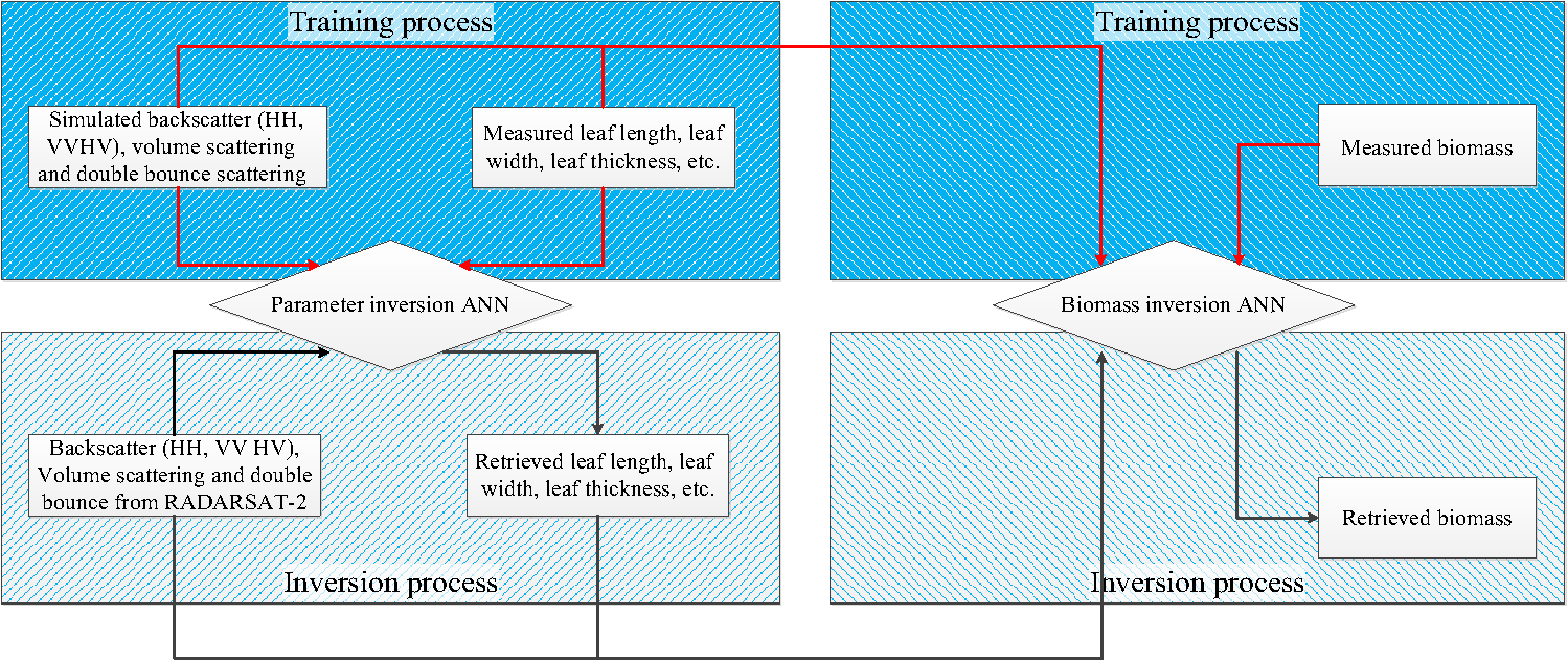

Here, the BP ANNs, standard feedforward multilayer perceptrons,²⁶ were used to retrieve the vegetation biomass (Fig. 7). The BP ANNs were both designed with two hidden layers. The number of neurons in the hidden layers was calculated according to $n=\sqrt{i\times j}+k/2$,⁴⁹ where $i$ and $j$ are the numbers of neurons in the input and output layers, and $k$ is the number of training samples. The transfer functions (activation function²⁶) for BP ANNs are the logarithm S transfer function {$a=\log \mathrm{sig}(n)=1/[1+\exp (-n)]$} and the linear transfer function [$a=\mathrm{pure}\mathrm{lin}(n)=n$]. The training function for BP ANNs is the “traingd” training function, which updates weight and bias values according to gradient descent.

4.1.

Biomass Inversion

First, the simulated volume scatter, double-bounce scatter, and backscatter for HH, VV, and HV polarizations obtained from the backscatter model were taken as the inputs, and the five surveyed VBPs were taken as the outputs to train the ANN. After training of this ANN, the Freeman polarimetric decomposition components (volume scatter, double-bounce scatter) and the backscatters for HH, VV, and HV polarizations from the RADARSAT-2 data were used to retrieve the biophysical parameters for the whole study area.

Second, the ANN for the biomass inversion was trained by use of the surveyed VBPs, the simulated volume, and double-bounce scatter as inputs and the biomass as output. By taking the retrieved VBPs and the Freeman polarimetric decomposition components (volume scatter, double-bounce scatter) from the RADARSAT-2 data as the inputs, the biomass for the whole study area was retrieved (Fig. 8).

Fig. 8

Biomass map retrieved from the RADARSAT-2 image.

The vegetation is mainly distributed along the shorelines on higher ground. The higher the elevation, the more biomass there is.

4.2.

Accuracy Assessment

The survey data consisting of the 54 samples were divided into two groups, one for training the ANN and the other for accuracy assessment. The accuracy of the wetland vegetation estimate was measured by use of the root-mean-square error (RMSE):

Eq. (2)

$$\mathrm{RMSE}=\sqrt{\sum _{}^{}{(B_e-B_g)}^2/n},$$

where $B_g$ is the biomass according to the ground truth, $B_e$ is the biomass according to the RADARSAT-2 PolSAR-based estimate, and $n$ is the number of observations.

The RMSE for polarimetric decomposition-based biomass inversion was $45.57\mathrm{g}/{\mathrm{m}}^2$, which is 13.06% of the average biomass ($348.8\mathrm{g}/{\mathrm{m}}^2$) obtained from the 54 surveyed data. The coefficient of determination, $R^2$, between the surveyed biomass and the retrieved biomass is 0.87 (Fig. 9).

Fig. 9

Comparison of model-simulated and field-measured biomass values.

5.

Discussion

For the Poyang Lake vegetated (mainly carex) wetland, the total backscattering is dependent on the interaction of the microwave energy with both the canopy and the canopy-ground. Both the characteristics of the canopy, such as density, distribution, orientation, shape of the foliage, dielectric constant, height, and branches and the characteristics of the sensor, such as polarization, incidence angle, and wavelength are important in determining the amount of radiation backscattered toward the radar antenna.⁵⁰

RADARSAT-2 PolSAR data appear to be well suited in mapping biomass in this area because the C-band (5.4 GHz) radar data are particularly sensitive to vegetation biomass when the canopy is above an underlying water surface or a water-saturated soil. This relation occurs because the dominant scattering mechanisms involve vegetation-water surface interactions.¹⁵ PolSAR data can provide more information for land cover classification and biomass inversion. The dependency of the polarimetric scattering features on the VBPs was investigated. Because of the distributed vegetation in the Poyang Lake wetland and the statistics feature around the field survey points, the incoherent Freeman polarimetric decomposition method was used to extract the polarimetric scattering features. The results confirm that the Freeman polarimetric decomposition components can be used to estimate the VBPs because of their sensitivity to the vegetation structure parameters.

Here, the backscatter model was used to analyze the relation between the backscatter and various VBPs. The results show that the backscatter model can be used to simulate the backscatter for wetland vegetation and to generate the training data for the ANN because wetland vegetation has the same structure as rice, for which the coefficients of determination are 0.93, 0.94, and 0.95 for HH, VV, and HV polarizations, respectively. However, SAR backscatter from vegetation-covered fields is a strong function of dielectric properties of the vegetation, vegetation canopy structure, vegetation volume along with moisture, and surface roughness of the underlying soil.^46,51,52 Sometimes SAR sensors may receive strong backscatter because of the double-bounce between the water surface and the vegetation stem.⁵³ Here, the soil properties were not considered in this study, because most of the sample locations were either flooded or oversaturated during image acquisition. Therefore, when the backscatter model is used to simulate the backscatter from vegetation, the backscatter will be underestimated because of the absence of the soil surface. The biomass will be wrongly estimated because of the assumption that the ground is covered by water in the backscatter model. If the ground soil was not flooded or oversaturated, the soil properties should be taken into account. If soil properties had been considered in the modeling process, the accuracy of the backscatter simulation and biomass inversion would have been expected to be improved. When the backscatter model is used, another factor that must be taken into consideration is the geometry (shape, size, geometric distribution, etc.) of the leaf. Here, the probability of geometric distribution function used in the model was adopted from Liu et al.,⁵⁴ where the vegetation and study area are the same types as in this study.

Because of the complex nonlinear relation between radar backscatter and wetland VBPs, the responses of scatter components to every single VBP show poor linear relation (Fig. 6). The occupied volume and moisture of each layer must both be taken into account for each layer when wetland VBPs and vegetation biomass are retrieved by use of SAR data.⁵¹ Here, the BP ANN was used to retrieve wetland VBPs and vegetation biomass because of the ability to express the nonlinear relation, which the traditional empirical and semi-empirical methods cannot do. When biomass was retrieved, the VBPs and the surveyed biomass were taken into account together. As a result, the ANN achieved good results, with $R^2$ on the order of 0.88 between the surveyed biomass and the retrieved biomass. However, the ANN was not optimized to the optimal solution, hence more work had to be done for the simulation and the optimization of the ANN. When remote sensing technology is used to retrieve vegetation biomass, the data source and methods influence the inversion precision to a great degree.⁵⁵ During training of the ANN, the upper and lower limits came from the survey data. Because they were not the actual values for the wetland vegetation, their use influenced the inversion accuracy.

The maximum values of vegetation biomass obtained during the field survey were $1650.1\mathrm{g}/{\mathrm{m}}^2$ (wet) and $348.8\mathrm{g}/{\mathrm{m}}^2$ (dry), which do not reach the saturation level for C-band SAR.³ The RMSE of overall biomass estimation for this area was better than that obtained by use of ENVISAT ASAR data in other studies.^11,54 The RMSE for polarimetric decomposition-based biomass inversion was $45.57\mathrm{g}/{\mathrm{m}}^2$, which is 13.06% of the average biomass ($348.8\mathrm{g}/{\mathrm{m}}^2$) obtained from the survey data. The coefficient of determination between the surveyed biomass and the retrieved biomass was 0.87 (Fig. 9).

6.

Conclusions

This study focused on the application of ANNs combined with a backscatter model to retrieve wetland vegetation biomass with RADARSAT-2 polarimetric SAR data. The backscatter model was used to analyze the relation between the backscatter and various VBPs. The results show that the Freeman polarimetric decomposition components are sensitive to the wetland VBPs and can be used to retrieve the VBPs for the Poyang Lake wetland. One trained ANN, taking the simulated backscatter, volume scatter, and double-bounce scatter as inputs and five VBPs as outputs, was used to retrieve the wetland VBPs. The retrieved VBPs, combined with polarimetric decomposition components from RADARSAT-2 data, were used to retrieve wetland vegetation biomass by use of another trained ANN. The RMSE for polarimetric decomposition-based biomass inversion was $45.57\mathrm{g}/{\mathrm{m}}^2$, which is 13.06% of the average biomass. The coefficient of determination between the surveyed biomass and the retrieved biomass was 0.87. The results indicate the potential for biomass estimation in wetland environments by use of a combination of PolSAR data, backscatter models, and ANNs.

A general problem with ANNs is the optimization, which influences the inversion accuracy, hence more work remains to be done. As far as the backscatter model is concerned, the soil status should be taken into consideration in subsequent work.