
|
|
1.IntroductionHigh-resolution remote sensing imagery has been used successfully in conjunction with image classification software tools for wetland vegetation mapping and wetland vegetation change detection for several decades.1–3 Wetland vegetation in general and seasonal wetland vegetation in particular exhibit high spatial and spectral variability because of steep environmental gradients, which produce short ecotones and often result in sharp borders between vegetated wetland regions.3–5 Spectral reflectance, the property of vegetation that is most often used to discriminate between important plant species of ecological significance, is a function of leaf optical properties that are related to the biochemical and physiological characteristics and health of the plant.3,6 Adam et al.,3 in a survey of spectral and multispectral survey techniques, acknowledge the complications with optical remote sensing techniques that perform classification based on spectral reflectance alone, given the similarities of spectral signatures and the potential interference from atmospheric conditions, plant moisture status, and underlying soil and litter characteristics. They provide examples of postprocessing techniques using fuzzy logic algorithms and other higher-order classification techniques that have been shown to improve classification accuracy. In addition to visible light and near-infrared (NIR) sensors that provide information about the surface chemical composition of vegetation and other materials, thermal infrared sensors measure near-surface thermal characteristics and radar sensors provide signals proportional to the near surface physical properties of topography, roughness, and moisture.7 Although hybrid optical and radar techniques might hold promise in the future for improving vegetation classification accuracy, there are few practical examples that might benefit the current study. The basic premise and motivation for the current study were to provide a quantitative assessment of potential long-term damage to wetland waterfowl habitat and to the overall wetland biological resource as a result of compliance with State-mandated salinity management objectives. Hence, the aim was to investigate whether quantitative longitudinal (over time) surveys of wetland moist soil plant succession, when combined with surveys of soil salinity, continuous monitoring of salts in and out of these wetlands, and biological monitoring of waterfowl and their food sources,8 could be used to help limit long-term damage due to wetland management practices such as delayed drawdown or other forms of water reuse. If shown to be accurate and reliable—vegetation mapping, in concert with these other survey techniques, could be used to provide assurances to seasonal wetland managers to embrace the concepts of real-time water quality management while promoting adaptive management of the biological resource. If this technology is to find widespread use in the Grasslands Basins wetlands, it also needs to be formulaic and easy to use. Given dwindling wildlife management agency budgets, it should also be relatively quick to perform and inexpensive. One potential cost-saving development might be the creation of spectral libraries for common wetland moist soil plant associations as suggested by Zomer et al.4 and Adams et al.3 This could considerably reduce the high cost of field surveys to verify the spectral signature of the most common and important moist soil plants. 1.1.BackgroundThe Grasslands Ecological Areas in California’s San Joaquin Valley constitute the largest contiguous wetlands remaining in California and provide essential habitat for migrating and overwintering waterfowl and shorebirds. They are recognized by RAMSAR as an ecological wetland resource of global significance. California wetlands have been significantly reduced in number and total area, largely through conversion to agricultural land. The loss of California wetlands since 1850 has been estimated at 91%, and in 1988, the California Department of Parks and Recreation estimated that California had lost 80% of its salt marshes and 90% of its freshwater marshes.9 The north Grassland Water District and San Luis National Wildlife Refuge (Fig. 1) together comprise of seasonal wetlands. These wetlands lie on the Pacific Flyway and are an important source of food and habitat for migrating and local bird populations. The wetlands, both publicly and privately owned, are also significant water users in the area. As water resources become increasingly scarce, the need to accurately estimate water needs and water quality impacts of these areas becomes an increasingly high-priority problem. The water regime in these managed wetlands is largely artificial, with surface water inflows and outflows designed to replace a natural wetland cycle. Water management practices include the timing of irrigation and drawdown to maximize desirable food production plants and to minimize undesirable weeds. Outflow events, such as wetland drawdown, can affect water quality in the San Joaquin River10—hence, wetland managers could schedule wetland drawdown to match periods of high San Joaquin River assimilative capacity. San Joaquin River assimilative capacity is determined by the salinity water quality objective at a downstream compliance monitoring station (Vernalis) and the ambient salt loading from upstream sources.11–13 The annual wetland salt load contribution to the San Joaquin River ranges from 8% to 11% of the total annual salt loading measured at the Vernalis compliance monitoring station.11,14 Fig. 1Project imagery (2004) showing North Grassland Water District (NGWD) outlined to the west and the San Luis National Wildlife Refuge (SLNWR) to the east. Inset shows the location of the site within central California. The image is displayed with a false color mapping and a contrast stretch to enhance viewability. Verdant vegetation displays as red in this mapping.  Modifications to wetland water management practices, such as changes in the scheduling of wetland spring drawdown, have the potential to alter the germination success of certain high yield and energetically important moist soil plants such as swamp timothy (Crypsis schoenoides), watergrass (Echinochloa phyllopogon), and smartweed (Polygonum hydropiperoides), which in turn can impact the wetlands’ ecological health and distribution of habitat.9,15–23 Historically, the hydrology of the Grasslands Basin wetlands was subjected to the local climate typified by cool, rainy winters and hot, arid summers. This resulted in a period of inundation during the fall and winter, followed by spring drainage and high rates of evapotranspiration during the summer months. The water regime in these seasonal wetlands is now extensively managed, with surface water inflows and outflows designed to replace the natural wetland hydrological cycle. Water management practices include the timing of flood-up, summer irrigation, and wetland drawdowns to maximize desirable food production plants and to minimize undesirable weeds. Habitat assessment is needed to optimize the timing of these changes. Traditional means of habitat assessment such as random sampling or transects for large areas () are extremely labor intensive.24 It can also be difficult to acquire timely data at a high enough resolution. Moreover, although impact assessment using a fine-scale sampling program at the individual pond level could be accomplished, the spatial variations found in larger areas may be missed completely. What is needed is a way to rapidly assess and quantify the various habitat communities at the regional scale and to readily track changes in those communities from year to year.25–36 Rapid and semiautomated methods of developing annual maps of important moist soil plants abundance and distribution using remote sensing are highly desirable. Investigating this possibility was one of the goals of this research. 1.2.Applications of Remote Sensing to Wetland Vegetation MappingMapping techniques that can accurately map large areas of seasonal wetlands are essential to the ability to manage the habitats, biodiversity, and other resources and services provided by wetland processes. Seasonal wetlands have been under-represented in attempts to map habitats using remote sensing. Although not all studies have been successful, high-resolution remote sensing has been demonstrated to have the potential to map wetlands at the species-level.25,26,28,32,33,36 The high spatial resolution of the sensor is essential to map the patchy distributions found in seasonal wetlands.37 Due to the high degree of vegetative diversity in seasonal wetlands, vegetation mapping is a challenging task. A maximum likelihood classification technique was initially chosen for image processing, since this algorithm effectively takes into account the covariance from other land cover classes. The application of polygon-based image processing techniques has been shown to be useful in reducing the noise created by pixel-based mapping and for helping to delineate areas of the wetland basins occupied by certain suites of species. The use of multitemporal imagery helps to distinguish vegetation classes that experience growth and reach peak maturity at different times—a feature of the vegetative community that is often characteristic of seasonal wetlands.19 Producing accurate vegetation maps of seasonal wetlands is a task with unique challenges. Like other wetlands, seasonal wetlands have a patchy distribution of vegetation that requires a high spatial resolution in order to map small and irregular shapes accurately. For this application, accuracy refers to the proportion of pixels for which their assigned land cover class correctly represents overstory vegetation or that seen by the aerial sensor. A number of wetland studies26,34,38 have found spatial resolution to be a limiting factor in their objective of mapping wetlands, even in the case of mapping broad classes that encompass a range of vegetation. Ozesmi and Bauer39 reviewed the use of low to medium resolution remotely sensed imagery, such as Landsat TM and SPOT, for mapping wetlands and found that the pixel size was one of the primary limitations. Other studies29,40 have successfully mapped wetlands’ extent and vegetation types using medium resolution satellites, but at the expense of detail in their land cover classes. Land cover classes in these two studies covered broad ranges, such as swamp, grasslands, crops, and shallow marsh, but did not attempt to discern vegetation associations within those classes. Seasonal wetlands have the potential to incorporate a great diversity of species, including species endemic to vernal pool landscapes.41,42 Although land cover classes may include more than one species, it is generally appropriate to represent a greater number of species with a greater number of land cover classes. While greater species richness in the landscape makes the task of mapping more difficult, the diversity of canopy structures exhibited by different species may pose some advantages. Different canopy structures can lead to different textures and can make visible varying amounts of soil, both of which may enhance variability in spectral reflectance between plant associations. Hyperspectral remotely sensed imagery offers some advantages over multispectral systems, but is more difficult to work with, more expensive, and less readily available.30 Time of year and environmental factors may also reduce its effectiveness. The reflectance spectra of a limited number of New Jersey salt marsh species were found to be separable using a handheld spectrometer in the fall.25 Schmidt et al.43 achieved only 40% accuracy using high-resolution hyperspectral imagery to map salt marshes in the Netherlands at the species level. Yang36 reviewed remote sensing studies of estuarine systems and found that the hyperspectral imagery had great potential for species discrimination, but that the implementation of hyperspectral studies is currently limited by a lack of spectral libraries available for wetland species. Hyperspectral imagery, such as ASTER with a ground-pixel size that varies from 15 m for VNIR, 30 m for SWIR, and 90 m for TIR can also be limited in its ability to map heterogeneous, patchy wetland environments. Hyperspectral imagery was used to map areas in Everglades National Park at the species level.30 However, the study’s success was limited by a lack of spatial resolution adequate to characterize irregular wetland patches. Few remote sensing studies of seasonal wetlands exist, so it is worth noting that Schmid et al.44 also used hyperspectral imagery in combination with ground spectra and multispectral imagery, to successfully map broad vegetation classes in seasonal wetlands in Spain. Using high-resolution multispectral imagery, such as IKONOS, Quickbird, or color infrared (CIR) aerial photography, has the potential to economically and accurately map wetland landscapes. Hurd et al.31 and Tuxen et al.45 used QuickBird data and CIR photography, respectively, to map salt marshes and found that accurate mapping at the species level was possible. In contrast, Shuman and Ambrose46 compared the use of high-resolution color infrared aerial photography to ground methods in identifying and quantifying land cover, including eight species, in a southern California salt marsh and found that, while CIR was an effective tool for judging percent ground cover, individual species could not be identified. As another example, an unsupervised clustering algorithm was applied to IKONOS imagery to classify broad classes of emergent and submergent vegetations in Minnesota wetlands.32 Preliminary results indicated that mapping at the species level was not possible with this combination of imagery and software. Furthermore, none of these project areas were comprised of the number of species typical of seasonal wetlands in California’s San Joaquin Valley. While pixel-based remote sensing has been the dominant paradigm for some time, recent developments in polygon-based, or object-based, image processing may improve mapping accuracies using high-resolution multispectral imagery.47 Polygon-based approaches correlate well with the human experience of the wetland landscape as patches of self-similar vegetation communities. Whiteside and Ahmad48 found the substantial benefit of polygon-based mapping when compared with pixel-based mapping of forested areas in northern Australia. However, only 10 broad vegetation classes were assessed in an area of over 1300 ha. Other researchers used information from both pixel-based and polygon-based classifications to map the extent of salt marsh in Long Island Sound using Landsat TM data.31 Preliminary results indicated that a hybrid pixel-polygon based approach improved the accuracy of their mapping. Remotely sensed digital imagery captures the spectral reflectance values of different land cover classes. By combining high-resolution satellite images and image processing tools with industry standard environmental survey methods, we can accurately and efficiently estimate the abundance of different species of wetland vegetation over large regions. Analysis of satellite imagery to quantify land cover in managed wetlands has multiple benefits. Compared with traditional vegetation survey techniques, satellite imagery requires significantly less time and labor, while covering a larger area. Rather than the exhaustive on-going field effort that would be required to survey a large area such as SLNWR, field work was limited to the time necessary to provide calibration for the image. While satellite imagery can be used effectively to map large or small areas, it becomes increasingly cost effective for larger study sites. Satellite imagery is also a flexible technology; depending on the variables of interest, image collection can be timed to capture different features throughout the growing season. Through tracking the changes in multitemporal imagery and correlating changes with previously made management decisions, impacts may be assigned to various land use activities.20 Satellite imagery is also an unbiased and consistent data source, reducing concerns of consistency between teams of surveyors, or drifts in field methodology and nomenclature during the field season. As an added benefit, the availability of satellite imagery as an unbiased and standardized data source creates the potential for study sites to be viewed in a broader context, both regionally and worldwide. Finally, the imagery provides an archival data source, which after its initial use continues to be available as a historical reference and can be used in later studies, the requirements of which may not have been foreseen at the time. 1.3.Application to San Joaquin Basin Seasonally Managed WetlandsIn this project, a methodology was developed for mapping seasonal wetlands in the San Joaquin Valley. The project was performed in two study areas: the San Luis unit of SLNWR and the northern zone of Grasslands Water District (NGWD). These two areas are in close association with similar climate, soils, and topology, yet they differ slightly in their management goals, land history, and diversity of both flora and fauna. The two areas represent two end points achieved through differing management strategies and provide the opportunity to evaluate the robustness of the mapping methodology. Mapping can perform two major functions for land managers of these areas: first to catalog the existing vegetation communities, both in composition and aerial extents; and second to assess changes in these communities over time. If a mapping methodology can perform these two functions conjunctively, it can provide valuable assistance to wetland managers in making effective management decisions. 1.4.Impacts of Basin Real-Time Salinity ManagementRecently enacted state water quality regulations for salinity in the San Joaquin Basin constrain the salt loading that can be returned to the river from all dischargers, including managed seasonal wetlands, so that it does not exceed the river’s assimilative capacity. Concentration objectives for salinity are to be met at a downriver compliance monitoring station primarily to protect water quality for Delta riparian agricultural diverters during the critical germination period. Average wetland salt loading currently accounts for between 10% and 15% of the total salt loading to the San Joaquin River, measured at the downstream compliance monitoring station.11 Real-time water quality management has been suggested as a means of improving the scheduling of wetland saline drainage loads to better coincide with periods of high assimilative capacity within the San Joaquin River.13,14,49 Delayed seasonal drawdown from private and public wetlands, managed for waterfowl habitat, is one option that is being considered so that the wetland drainage salt loads are scheduled to coincide with reservoir releases of high-quality water, made annually in the spring to aid salmon migration. Real-time water quality management would require that a sufficient volume of wetland saline drainage be rescheduled to help meet water quality objectives—this annual volume could be large in dry and critically dry water years and small or zero in wet water years. Real-time water quality management will only be successful if actions such as delaying seasonal wetland drawdown or wetland drainage reuse can be shown to have no long-term impact on the habitat value, biological health, and diversity of the seasonal wetland resource for migratory waterfowl and shorebirds. Potential long-term impacts of making changes to the traditional scheduling of seasonal wetland drawdown are being assessed in this and related projects using both biological and vegetative survey techniques. In this paper, only vegetation mapping aspect of this larger resource management study is discussed. 2.Methods2.1.ImageryThe QuickBird satellite (Digital Globe, Longmont, Colorado) was tasked to provide high-resolution, multispectral imagery for the project. A high spatial resolution was necessary to capture the spatial variability of the patchy and irregularly shaped vegetation communities that are typical of these wetlands. Mapping for this project was conducted using this digital high-resolution remotely sensed imagery—each subsequent year of imagery is being compared with a base year as a means of detecting change conditions.50 The imagery provided bands in the blue, green, red, and NIR spectrum. The imagery was orthorectified by Digital Globe, and the root mean square error for the orthorectification process was 2.1 pixels. Objects reflect solar irradiance with respect to their individual spectral and directional properties. Radiometric correction of images is performed to take account of various atmospheric distortions to surface reflectance and becomes necessary when imagery from different dates and sensors is used for quantitative image analysis. No radiometric or reflectance corrections were performed on the imagery for two reasons: (a) the imagery was collected from the same sensor and taken at approximately the same time of day; and (b) our aim was to develop a low-cost and technically manageable solution—performing these corrections would have beyond the skill of the analysts targeted in the study. Imagery was collected for three dates—April 26, May 14, and June 19, 2004. Image collection was timed to capture different stages of growth throughout the growing season. Image pixels were assigned vegetation classes based on the dominant land cover class. Land cover classes used in this study may be comprised of buildings, open water, bare soil, litter, or a particular association of vegetation. The late April image would capture seedlings and perennials in wetland basins and verdant uplands vegetation. The May imagery was timed to coincide with the maximum growth period for the wetland basins, following the first summer irrigation, usually late May to early June.51 The May imagery would, therefore, capture a mix of inflorescence and mature growth in the wetland basins and a mix of inflorescence, verdant growth, and seeding in the uplands vegetation. The June imagery was chosen to capture inflorescence, mature growth, seeding in the wetlands basin, and seeding and senescence in the uplands vegetation. 2.2.Ground Sampling SurveysFor field data collection, a novel Rapid Assessment Protocol (CNPS-RAP) recently developed by the California Native Plant Society was modified to more accurately represent the wetland moist soil plant community structure. The CNPS-RAP employs a community-based approach to surveying and provides a methodology for collecting basic quantitative information sufficient for identification and verification of habitats. In its original format, the CNPS-RAP uses a one-page worksheet to rapidly assess large landscapes for a number of important parameters. These parameters include location and distribution of vegetation types and communities, composition and abundance information on the member plant species, and general site environmental factors. The CNPS-RAP also provides guidance for the identification of plant community characteristics such as the level of community disturbance.52 This method has been used to provide land use managers with efficient tools for natural resource inventorying and planning.52 Modifications were made to the published CNPS protocol to make it applicable to our study—this protocol had not previously been applied to seasonally managed wetlands. For example, in our field surveys, field protocols ignored the CNPS’s emphasis on native species and placed equal weight on cataloging important non-native species (Table 1). Because of the availability of detailed soils maps for the area, the time-consuming soil classification technique used by the RAP was replaced by existing soil survey data. Other minor modifications included the addition of new data fields, such as annotating the presence of visible salts, as it was perceived that this could have an effect on the spectral response of the land cover. The traditional RAP vegetation worksheet was programmed into a handheld GPS computer. Parameters collected include composition and abundance information on the sampling locations’ plant species, their state of health, and growth stage. General site environmental factors were also tabulated including litter cover, anthropogenic disturbances, the presence of visible salts, and soil cracking. No particular emphasis was placed on cataloging native species for this study. Table 1Sample field data from modified California Native Plant Society Rapid Assessment Protocol (CNPS-RAP).
A Trimble GeoExplorer 3 GPS was programmed with the data fields necessary to define a vegetation community. Data were postprocessed via differential correction to improve on-ground accuracy to less than 2 m. Modified RAP data representing a community of vegetation were associated with a single point on the map. Field personnel worked in teams defining the boundaries of a homogenous area, visually estimating the size and shape of the area, and then characterizing it according to the field protocol. Sampling locations represent all managed, accessible ponds in the San Luis Unit. (The southwest corner of the refuge is home to a sensitive species, the tule elk, and was not sampled for that reason.) Local biologists assisted field personnel in stratifying data collection efforts so that the common associations were well represented. More emphasis was placed on sampling wetland basins than upland areas. A total of 407 samples were collected during the weeks surrounding imagery collection. Figures 2 and 3 show the sampling locations overlaid on project imagery. Fig. 2Ground truth locations, San Luis Unit, San Luis National Wildlife Refuge, Merced County, California. Field data locations have been overlaid on a false color mapping of the near-infrared (NIR), red, and green bands of the May 14, 2004, satellite imagery. Regions of verdant vegetation appear red, water appears dark, and regions of dry uplands appear light green.  Fig. 3Ground truth locations, Salinas Club, Merced County, California. Field data locations have been overlaid on a false color mapping of the NIR, red, and green bands of the May 14, 2004, QuickBird imagery. Regions of verdant vegetation appear red, water appears dark, and regions of bare, dry soil appear bright. 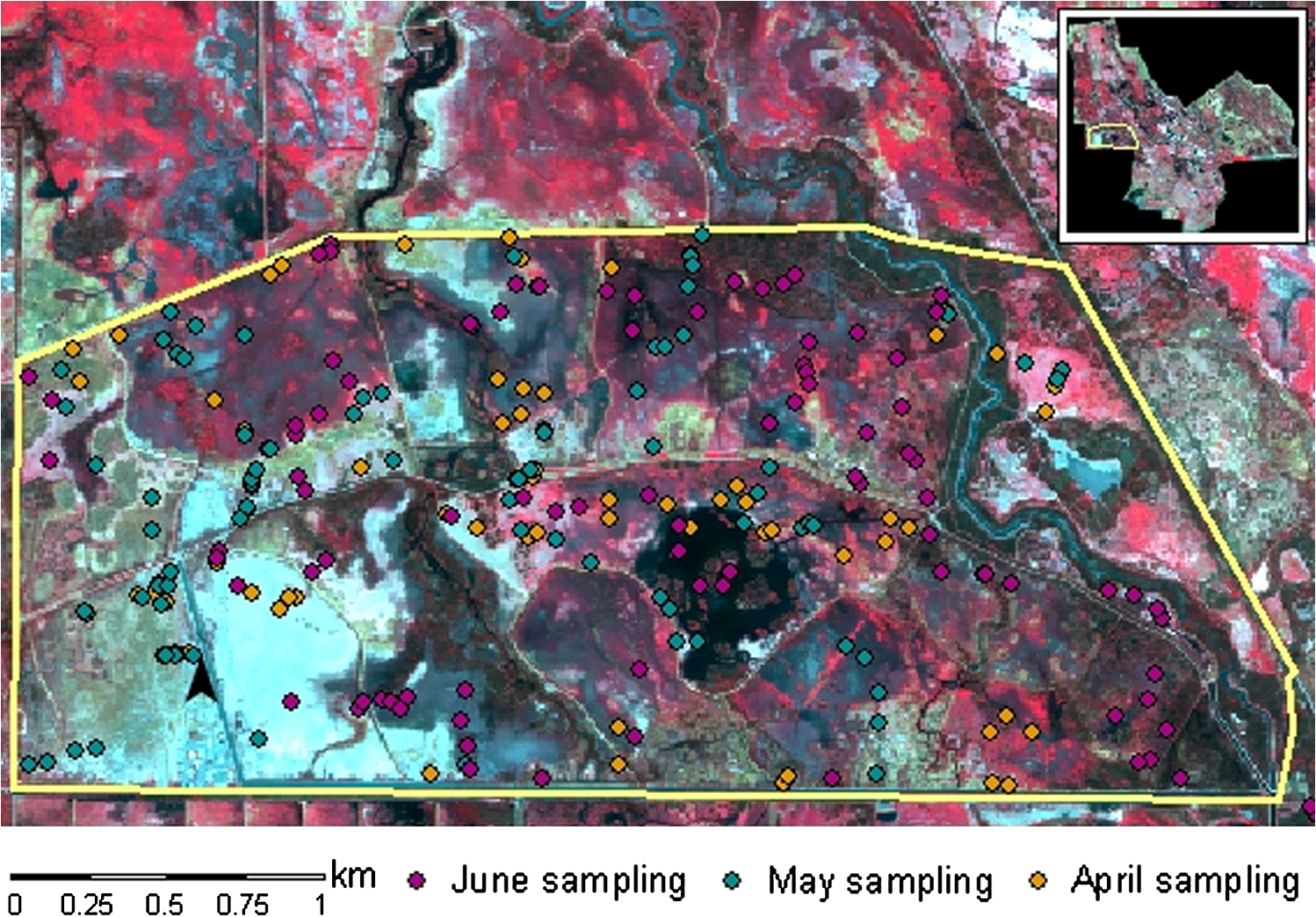 2.3.Ground Truthing SurveysGround truthing of remotely sensed imagery is the process of collecting in situ data that tie the spectral values in the imagery to land cover on the earth’s surface. Ground truth data may be used both as input to the classification process and, once classification is complete, to check the accuracy of interpretation. Ground truth data were collected during the days shortly before, during, and after the satellite flyovers to ensure maximum correlation between field data and the recorded image. Ground truth data were collected on the San Luis Unit of the SLNWR and from the Salinas Land and Cattle Club (Salinas Club), a privately owned area of approximately 600 ha, during the same time period. Ground truth data were postprocessed for improved accuracy and utility. GPS feature positions were postprocessed via differential correction to improve the accuracy of feature locations. Differential correction utilizes data from a regional base station with a known, fixed location to correct for GPS errors that may be introduced via satellite error, transmission error, or atmospheric effects. Differential correction was performed using Trimble Pathfinder Office software and using cotemporaneous base station data from the National Geodetic Survey Continuously Operating Reference Stations. Following differential correction, the data were exported to ESRI (Redlands, California) shapefile format. The feature attribute data were then analyzed using ESRI’s ArcGIS software to identify the two dominant species in each vegetation community. The field data could then be applied to classification of the images. In a few cases, ground truth points were selected after the fact based on the analyst’s interpretation of the images. Data points were selected this way for the land cover classes of trees, water, and buildings. Each of these land cover types was easily identifiable through visual analysis of the image and difficult to obtain values for in the field. Collecting points in this way involves a negligible risk of error on the part of the analyst and ensures adequate data to compile a robust spectral signature for these classes. 2.4.Classification SchemaPixels and ground truth points were assigned to 1 of the 20 land cover classes. Vegetation land cover classes were developed from observations of the dominant species in each vegetation assemblage at ground sample points. Land cover classes are listed in Table 2. The decision to combine two or more dominant land cover classes into a single class was based on the similarity of their habitat, the frequency of their co-occurrence on the landscape, and the amount of spectral confusion between the classes that was observed in the check point dataset. For example, alkali heath, alkali weed, dwarf spikerush, and bare soil all occur in similar habitats and often co-occupy the same habitats. There was significant spectral confusion between these four classes. Table 2Land cover classes, abbreviations, and data points.
The complexity of the seasonal wetland landscape intensifies the difficulty inherent in developing a representative classification schema. The 20 land cover classes in this schema do not represent the entire diversity of plant species that exists in these wetlands. Rather, it represents the most commonly observed dominant plant species. Recorded observations commonly noted three to five additional plant species as members of the vegetation community at most ground truth points. A number of plant species exist widely as minor characteristics of the landscape, but rarely or never outnumber other proximal species. In particular, a small number of vegetation communities dominated by mustards (Brassica spp.), poison hemlock (Conium maculatum), chufa (Cyperus esculentus), atriplexes (Atriplex spp.), burhead (Echinodorus berteroi), dodder (Cuscuta brachycalyx), calicoflowers (Downingia spp.), mallows (Malva spp.), and others were observed in the landscape. However, an insufficient quantity of field data was collected to formulate spectral signatures for these communities. Although vegetation communities dominated by these species will necessarily be misclassified, they are estimated to cover less than 1% of the landscape. A priori knowledge of the abundances and dominant status of different species can improve the development of the classification schema, the effective deployment of field resources, and classification accuracies. In the present study, cattails, curly dock, tules, spikerush, water hyacinth, and litter were described by an undesirably small number of training areas. Water hyacinth was judged to have a sufficiently distinct spectral signature that it could effectively be represented by only a few points. In the case of the other five under-represented land cover classes, they were observed to comprise a large area of the landscape, and hence could not be left out of the classification schema. 3.Results3.1.Image ProcessingAfter the training area was defined, the image processing software was used to compile statistics that describe the pixel spectral values. This process was repeated until a signature for each ground truth point was created to be used as a training area. The final result was a compilation of 262 spectral signatures used by the classification algorithm. An estimated probability of appearing in the landscape was assigned to each spectral signature prior to classification processing. Estimated probabilities were based in part on field personnel observations and in part on prevalence of that land cover class in the collected field dataset. ERDAS automatically normalizes the sum of the probabilities for the 262 signatures so that they sum to 100%. 3.2.Pixel-Based Image Processing and ClassificationPixel-based image processing and data analysis were performed using software routines provided by ERDAS Imagine Professional. Other off-the-shelf commercial image processing packages are available that perform comparable analyses. A supervised classification technique—whereby data input by an analyst is used to determine seed values for classes—was selected for classification of the images. Maximum likelihood classification is a standard industry algorithm for projects where adequate ground truth data have been collected. This technique requires the input of “training” data, with which software algorithms define statistically based spectral bounds for each class. Training data are derived from ground truth points, once an area around each ground truth point representative of that community of vegetation has been defined—the image processing software compiles statistics that uniquely describe the spectral values for that community. Multiple ground truth points were combined into a robust spectral signature for a single land cover class, and this process was repeated until a signature was created for all desired land cover classes. After all training data were entered into the spectral signature file, the classification algorithm was implemented. The maximum likelihood algorithm uses the defined spectral signatures to extrapolate from the training pixels to all the pixels in the image. This is an efficient process, resulting in the use of data from a few thousands of pixels to classify an entire image comprised of tens of millions of pixels. Every pixel was assigned to a class—the class it is “most likely” to belong to, even if the pixel’s spectral values fell outside the initial seed values for that class. Through a complex process of signature refinement, individual training signatures (Fig. 4) evolve into the final class signature file that is used to classify the image. The class signatures are based on multiple single signatures added together in proportion to the number of pixels each represents. After signatures are compiled for each class, they may be evaluated for separability. There are several tools that may be used for this evaluation. Figure 5 shows a matrix of separability values for 10 land cover classes. The matrix shows the separability of pairs of classes. For example, the value in row 1 and column 2 would indicate an excellent separability between Scirpus spp. and bare soil/iodine bush. Classes that are not adequately separable can result in pixels misclassified as the other member of the pair. Separability was calculated in all four image bands, using a measure of the spectral distance between classes known as transformed divergence. Transformed divergence ranged in value from 0 to 2000, and values over 1500 were considered to be separable. Fig. 4May 14, 2004, spectral signature file. Each class is the result of compositing training data for numerous ground truth points. The total number of pixels included in each class is displayed in the “Count” column. The color swatch, used for visualization only, is derived from the average values of all pixels comprising that class, based on the color mapping used in the display window. Since NIR is mapped to red in the display window, vegetation tends to appear red.  Fig. 5Separability matrix showing transformed divergence values for the first 10 land cover classes from the spectral signature file. Values over 1900 are considered to indicate excellent separability; values greater than 1700 represent good separability; and values greater than 1500 are considered adequately separable. 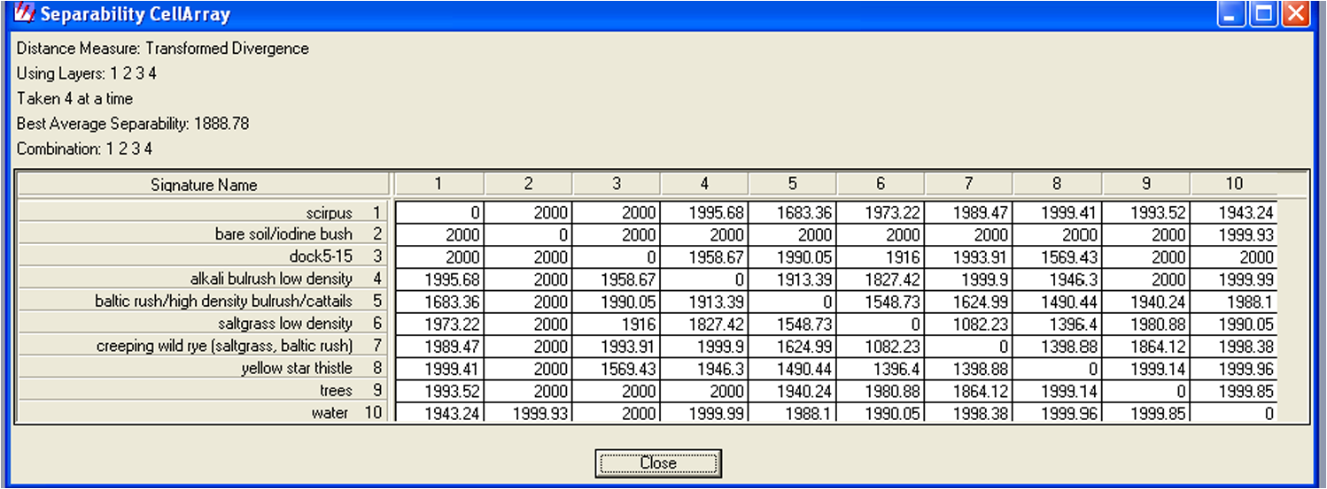 3.3.Object-Based Image Processing and ClassificationDefiniens eCognition software is an advanced, object-based image processing package providing specialized algorithms not currently available in traditional (pixel-based) image processing packages. For the purposes of this project, eCognition was used in conjunction with ERDAS Imagine Professional to apply a maximum likelihood classification to landscape objects in the form of polygons. eCognition uses spectral and shape characteristics of the raw imagery to separate pixels into self-similar landscape objects. This correlates well with viewing the landscape in terms of vegetation communities or in terms of homogenous land cover classes such as roads or water. Polygon objects created using eCognition were used later in the study to compare a landscape-object-based approach to a pixel-based approach in using the maximum likelihood classifier. A close up of the raw imagery divided into landscape object polygons is shown in Fig. 9. In Fig. 6, band 2 (green) is plotted on the -axis, and band 4 (NIR) is plotted on the -axis. The two-dimensional location of a point on this plot is determined by its spectral value in the two bands. Colors represent the frequency of occurrence of that spectral value combination. Red depicts the combinations that occur frequently in the dataset. Violet depicts the combinations that occur least frequently. The class bounds, as determined by training data, of buildings, Scirpus spp., and water are plotted on this feature space. The three classes are unambiguously separable in bands 2 and 4. Furthermore, buildings occupy a sector of feature space not represented in too many pixels. Scirpus spp., by contrast, is centered around a red sector. This could indicate either a predominance of Scirpus in the image or a predominance of land cover classes that reflect a signal similar to Scirpus spp. Fig. 6Feature space analysis of separability of three land cover classes in bands 2 and 4 of the May 14, 2004, imagery.  An object-based vegetation map was developed for the May 14, 2004, imagery. An object-based map was created by using a zonal analysis method to synthesize the results of the pixel-based maximum likelihood classification with the landscape objects created via eCognition. Landscape objects incorporated spectral and shape information from the April, May, and June imagery and used an eCognition scale factor of 50 (Fig. 7). Polygons were assigned a land cover class based on the plurality of pixels existing within each polygon. The result is a smooth, more easily interpretable vegetation map (Fig. 8) which improves the classification accuracy for some classes. Fig. 7Segmentation of imagery into self-similar polygon objects. Blue dots represent a hypothetical spectral signature of each cattails training area, and the orange circle represents the hypothetical spectral region in which pixels would be assigned to the Ty spp. class.  Fig. 8Pixel-based maximum likelihood classification of the Grasslands Basin wetlands that includes both the SLNWR and NGWD. 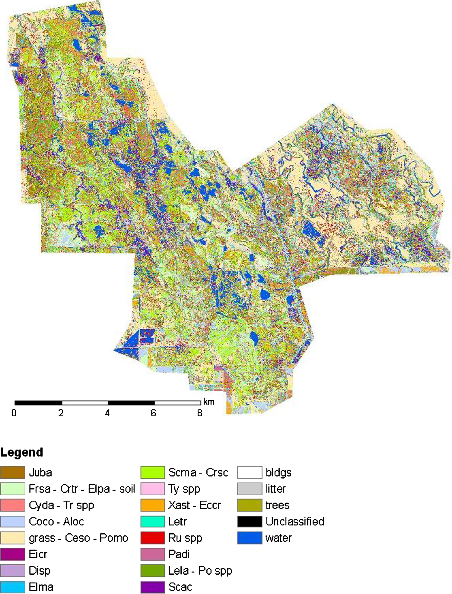 Polygon objects were used to compare a landscape-object-based approach to a pixel-based approach. Maximum likelihood classification assigns each pixel to a land cover class. Within each polygon object, the number of pixels assigned to each class was tallied and the polygon was assigned to the land cover class owning the most pixels in that polygon. This reduced noise in the classification and created a generalized map useful for calculating the extent of different land cover classes. 3.4.Image Processing Accuracy AssessmentAccuracy assessment was performed through standard calculations using randomly selected ground truth points that had been set aside especially for this purpose. Check points are not used in creating training signatures—hence they are a reliable, independent dataset for classification verification. The number of check points was 79, 115, and 131 for April, May, and June, respectively, for the mapped areas. Accuracy assessment was evaluated using two industry-standard metrics: producer’s accuracy and user’s accuracy. Producer’s accuracy is the ratio of the number of correctly classified check points in a class to the total number of reference check points in that class. User’s accuracy is the ratio of the number of correctly classified check points in a class to the total number of reference check points that were classified as the target class. This metric is a measure of commission error and represents how likely it is that an imagery pixel assigned to that class is actually a member of that class. Error matrices display both errors of commission and omission as shown in Tables 3 and 4. Numbers in the diagonal represent a correctly classified point. The producer’s accuracies, displayed in the far right column, are a ratio of the number of correctly classified check points to the number of check points collected in that land cover class. This is a measure of how correctly check points in that class are classified. The user’s accuracies, displayed in the bottom row of the matrix, are a ratio of the number of check points in a class that were correctly assigned to the total number assigned to that class. This is a measure of how likely a pixel assigned to that class on the final map will be correct.53 Table 3.Error matrix for pixel-based maximum-likelihood classification of the Grassland Basin wetlands.
Note: Overall accuracy: 60%. Table 4Error matrix for polygon-based maximum-likelihood classification of the Grasslands Basin wetlands.
Note : Overall accuracy: 54%. The overall mean accuracy obtained in mapping land cover through a pixel-based method was 60% (Table 3), with the error seen in individual classes ranging from 0% (Ty spp. and litter) to 100% (Juba, bldgs, Scac, and Eicr). The overall accuracy is computed as the number of correctly classified points divided by the total number of check points. Classes that achieved a user’s mapping accuracy of 75% or better include Frsa—Crtr—Elpa—soil, Juba, bldgs, Scac, Xast—Eccr, water, and Eicr. In addition, substantial confusion exists between the two closely related classes Crsc—Scma (swamp timothy and alkali bulrush) and Frsa—Crtr—Elpa—soil (alkali heath, alkali week, dwarf spike rush, and bare soil). Considering the functioning of these two classes in the context of the wetland ecosystem, it would be reasonable to combine these two classes, resulting in a higher level of accuracy for both classes and a higher overall accuracy for the classification. In contrast, the maximum likelihood classifier clearly had difficulty distinguishing the following classes: Ty spp., Letr, Ru spp., Padi, and litter. From field observations, Ty spp. (cattails), Ru spp. (curly dock), and litter all exist in a myriad of forms. Cattails exist on the landscape as both a sparse and dense dominant, allowing a bird’s eye view of a wide range of soil and understory plants. Curly dock coexists with a broad range of commensurals, from upland to emergent species. Finally, litter ranges from a whitish algal litter, to gray woody stems, to brown senescent leaf litter. These three land cover classes would be well served by a greatly increased number of training points and check points to characterize each of them. Padi (jointgrass) was not observed to be highly variable, but may also benefit from collection of additional ground truth points. The polygon-based mapping (Table 4) achieved an overall accuracy of 54%. For the polygon-based method, user’s accuracies for individual classes ranged from 0% (Ty spp. and Rum spp.) to 100% (buildings and Eicr). These results imply that a polygon-based approach for classifying wetland imagery may produce less accurate maps than a pixel-based approach. However, during processing of the imagery, some further improvements to the process became clear. In future work, it would clearly be desirable to collect each training area from a multitemporal image. For example, in this case, the spectral information for training areas could be derived from a 12-band image including blue, green, red, and NIR bands from the April, May, and June images. This would clearly provide additional data to the classifier which might be very beneficial in separating different land cover classes. A map of moist soil plant vegetation for the Grasslands Basin wetlands based on pixel-based maximum-likelihood classification is shown in Fig. 9 and for the polygon-based maximum-likelihood classification in Fig. 10. There is very little difference visible to the eye. Figures 11 and 12 are more detailed version of these same maps, which zoom in to just the SLNWR area. The visual appearance of the maps is quite distinct with more obvious clustering of moist soil plants in the polygon-based map. Figure 12 shows how moist soil plant vegetation changes between the months of May and June. The most obvious change in the June imagery (pixel-based processing) is in the abundance of watergrass—which is a forb favored by late pond drawdown and which is one of the three main protein sources for over-wintering waterfowl. Fig. 9Polygon-based maximum-likelihood classification of the Grasslands Basin wetlands that includes both the SLNWR and NGWD. 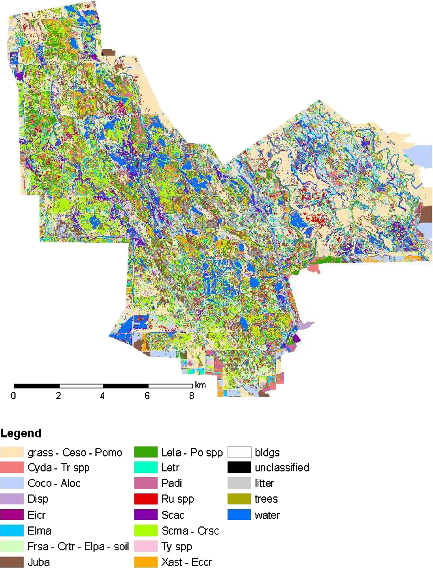 Fig. 10May 14, 2004, maximum likelihood pixel-based classification of the SLNWR. The map shows in more detail the transitions between the moist soil plant associations.  4.DiscussionA primary objective of this study which was to develop remote sensing as a component resource assessment technology to support other monitoring programs to advance the concept of real-time salinity management in the San Joaquin Basin of California was realized. Other ongoing resource assessment programs include: (a) monitoring sensor networks to continuously measure flow and electrical conductivity of water entering and draining from a selected set of 18 wetland impoundments; (b) soil salinity mapping of the same wetland impoundments using electromagnetic sensor technologies (Geonics EM-38); (c) annual clip surveys to assess biomass and seed production for swamp timothy (C. schoenoides) in the impoundments; and (d) waterfowl use surveys to indirectly assess changes in habitat function. Use of the hybrid pixel- and object-based optical remote sensing techniques for wetland habitat assessment and change detection proved cost-effective and provided valuable information in a form useful to wetland managers. The suggestion from the published literature3,4 that the spectral signals could be developed in a library for common wetland moist soil plant associations which would remain stable with time proved elusive. In the succeeding three years (2005 to 2008), during which imagery was either obtained from satellite or from aerial images, there were significant changes in the composition of these associations. As the mix of forbs or other moist soil plants in these vegetation associations changes, so does the spectral signature. Hence, a full-field campaign of ground sampling would be required each year to obtain accurate and meaningful results. Field work for this study was performed without the benefit of prior knowledge of the abundance or distribution of species. Field work was also constrained by time and limited personnel. In these seasonal wetlands, annual emergent vegetation cannot be located until late spring, when winter irrigation has subsided and seeds have had enough time to germinate. The later end of the growing season is so hot and dry that most annuals have reached senescence by early July. After senescence, it was more difficult to distinguish different vegetation communities. A highly targeted field season was necessary to collect adequate data for classification of the large number of land cover classes. By using the land cover map created from 2004 data, later data collection efforts were better able to stratify data points between classes and reduce bias by employing randomization of data point collection. Less effort was devoted to collecting data representing alkali bulrush, swamp timothy, alkali heath, alkali weed, dwarf spikerush, and bare soil, while more effort was devoted to classes exhibiting lower classification accuracies. Implementation of real-time water quality management in the San Joaquin Basin aims to improve coordination of saline wetland drainage return flows to the San Joaquin River with River assimilative capacity for salt. Concerns over the long-term impact of salinity management applied to seasonal wetlands which could require practices such as delays to scheduled wetland drawdown were the motivation for this study—to compare and contrast moist-soil plant vegetation succession in wetlands managed traditionally and those subjected to delayed drawdown. The study focused on the development of analytical mapping techniques for moist soil plant association mapping using two state-of-the-art software packages—ERDAS Imagine (Leica Geosystems) and eCognition (Definiens). These mapping techniques used a combination of pixel- and polygon-based image processing procedures. Twenty-six different plant communities were represented in a total of 20 land cover classes. An overall mapping accuracy of 60% was achieved for characterization of the 26 moist soil plant association classes and over 75% for the characterization of individual plant species. Given the complexity of moist soil plant vegetation within seasonally managed wetlands–it is expected that some land cover classes would be mapped at very high accuracies and other land cover classes at very low accuracies.54 In general, buildings and bare soil were readily and successfully discriminated using the digital classification techniques deployed. Certain types of vegetation with overlapping spectral signatures were often difficult to tell apart. Error assessment was compromised by certain wetland moist soil plant associations where sample sizes used for classification and error assessment were significantly different (they should ideally be of the same size). In one instance, only a single instance of a particular moist soil plant association was recognized making statistical assessment impossible. 5.ConclusionsThe results of this mapping endeavor produced the first comprehensive seasonal wetland vegetation maps developed for this region. The results suggest that these techniques have great potential for future wetland resource management as modified wetland drawdown and other real-time salinity management practices are considered as ways of complying with state discharge water quality regulations. Future improvements can potentially be made to the method through full utilization of multitemporal high-resolution imagery and improved stratification of data collection across land cover classes. One innovation presented in this paper was the adaption of a rapid vegetation assessment protocol (CNPS-RAP) developed by the California Native Plant Society55 and currently used throughout California. Our adaption involved the substitution of many upland vegetation plant associations with moist soil plant association more typical of wetland habitat. The second innovation resulted from our comparison of pixel- and object-based imagery processing techniques for both ease of use and accuracy and our refinement of a hybrid approach that improved efficiency and repeatability at a relatively low cost. One major change that has occurred since the study was concluded in 2008 has been the free access to Landsat imagery and a significant reduction in the cost for higher resolution imagery from privately owned satellites. Keeping costs down will be essential if change detection remote sensing is to become an integral component of the real-time salinity management program. AcknowledgmentsThe authors are indebted to the State Water Resources Control Board, US Bureau of Reclamation and California Department of Water Resources for grant funding in support of this ongoing research. Thanks also to the Grassland Water District, Salinas Land and Cattle Club, California Department of Fish and Game, and U.S. Fish and Wildlife Service on whose lands the study was been carried out. Of particular note is Jeff Milliken (US Bureau of Reclamation), who provided technical assistance on ERDAS Imagine and Definiens eCognition modeling, Tim Poole (Salinas Land and Cattle Club) for his help in vegetation identification, and Ricardo Ortega and Lara Sparks (California Department of Fish and Game), who assisted with various aspects of field data acquisition, vegetation surveys, and ground truthing. This research was also supported by the U.S. Department of Energy and LBNL under Contract No. DE-AC02-05CH11231. ReferencesX. Huang et al.,
“New postprocessing methods for remote sensing image classification: a systematic study,”
IEEE Trans. Geosci. Remote Sens., 52
(11), 7140
–7159
(2014). http://dx.doi.org/10.1109/TGRS.2014.2308192 IGRSD2 0196-2892 Google Scholar
R. Pu and S. Landry,
“A comparative analysis of high spatial resolution IKONOS and WorldView-2 imagery for mapping urban tree species,”
Remote Sens. Environ., 124 516
–533
(2012). http://dx.doi.org/10.1016/j.rse.2012.06.011 RSEEA7 0034-4257 Google Scholar
E. Adam, O. Mutanga and D. Rugege,
“Multispectral and hyperspectral remote sensing for identification and mapping of wetland vegetation: a review,”
Wetlands Ecol. Manage., 18
(3), 281
–296
(2010). http://dx.doi.org/10.1007/s11273-009-9169-z WEMAEU 0923-4861 Google Scholar
R. J. Zomer, A. Trabucco and S. L. Ustin,
“Building spectral libraries for wetland land cover classification and hyperspectral remote sensing,”
J. Environ. Manage., 90 2170
–2177
(2009). http://dx.doi.org/10.1016/j.jenvman.2007.06.028 JEVMAW 0301-4797 Google Scholar
K. S. Schmidt and A. K. Skidmore,
“Spectral discrimination of vegetation types in a coastal wetland,”
Remote Sens. Environ., 85 92
–108
(2003). Google Scholar
J. C. Price,
“Variability of high resolution crop reflectance spectra,”
Int. J. Remote Sens., 13 2593
–2610
(1992). http://dx.doi.org/10.1080/01431169208904066 IJSEDK 0143-1161 Google Scholar
E. Elachi and J. Van Zyl, Introduction to the Physics and Techniques of Remote Sensing, 2nd ed.Wiley-Interscience, John Wiley and Sons, Hoboken, New York
(2006). Google Scholar
K. J. Reinecke and K. M. Hartke,
“Estimating moist-soil seed available to waterfowl with double sampling for stratification,”
J. Wildl. Manage., 69
(2), 794
–799
(2005). http://dx.doi.org/10.2193/0022-541X(2005)069[0794:EMSATW]2.0.CO;2 JWMAA9 0022-541X Google Scholar
W. R. Ferren, P. L. Fiedler and R. A. Leidy,
“Wetlands of the central and southern California coast and coastal watersheds: a methodology for their classification and description,”
(1995). Google Scholar
“Lower San Joaquin River water quality investigation,”
(1969). Google Scholar
“Amendments to the water quality control plan for the Sacramento and San Joaquin River Basins for the control of salt and boron discharges into the San Joaquin River,”
(2003). Google Scholar
“Total maximum daily load for salinity and boron in the lower San Joaquin River,”
(2002). Google Scholar
N. W. T. Quinn et al.,
“Computer model improves real-time management of water quality,”
Calif. Agric., 51
(5), 14
–20
(1997). http://dx.doi.org/10.3733/ca.v051n05p14 CAGRA3 0008-0845 Google Scholar
N. W. T. Quinn and W. M. Hanna,
“A decision support system for adaptive real-time management of seasonal wetlands in California,”
Environ. Modell. Software, 18
(6), 503
–511
(2003). http://dx.doi.org/10.1016/S1364-8152(03)00025-2 EMSOFT 1364-8152 Google Scholar
R. M. Bundy,
“Hydrology influences on vegetation response in a managed moist-soil impoundment,”
University of Missouri-Columbia,
(1997). Google Scholar
“Ecological and water management characterization of Grassland Water District,”
(1986). Google Scholar
L. F. Grober, K. Karkoski and T. Poole,
“Water quality impact of wetlands on San Joaquin River, California, paper no. 00149,”
in Advances in the Development and Use of Models in Water Resources: Proceedings of the American Water Resources Association,
(1995). Google Scholar
E. Burns, M. Miller and J. Eadie,
“An analysis of food habits of Green-Winged Teal, Northern Pintails, and Mallards wintering in the Suisun Marsh to develop guidelines for food plant management,”
(2003). Google Scholar
S. Fennessey et al.,
“Methods for evaluating wetland condition: using vegetation to assess environmental conditions in wetlands,”
(2002). Google Scholar
L. Fredrickson,
“Strategies for water level manipulations in moist-soil systems,”
Waterfowl Management Handbook, 1991). Google Scholar
K. S. Gilmer et al.,
“California’s Central Valley wintering waterfowl: concerns and challenges,”
Trans. North Am. Wildl. Nat. Resour. Conf., 47 441
–452
(1982). NAWTA6 0078-1355 Google Scholar
H. L. Mason, A Flora of the Marshes of California, 879 University of California Press(1969). Google Scholar
W. D. Smith, G. L. Rollins and R. L. Shinn, A Guide to Wetland Habitat Management in the Central Valley, 34 California Dept. of Fish and Game, California Waterfowl Association, Sacramento, California
(1995). Google Scholar
O. W. Taft et al.,
“Waterbird responses to experimental drawdown: implications for the multispecies management of wetland mosaics,”
J. Appl. Ecol., 39 987
–1001
(2002). http://dx.doi.org/10.1046/j.1365-2664.2002.00763.x JAPEAI 1365-2664 Google Scholar
F. J. Artigas and J. Yang,
“Spectral discrimination of marsh vegetation types in the New Jersey Meadowlands, USA,”
Wetlands, 26 271
–277
(2006). http://dx.doi.org/10.1672/0277-5212(2006)26[271:SDOMVT]2.0.CO;2 0277-5212 Google Scholar
S. Berberoglu, K. T. Yilmaz and C. Ozkan,
“Mapping and monitoring of coastal wetlands of Çukurova Delta in the Eastern Mediterranean region,”
Biodiversity Conserv., 13 615
–633
(2004). http://dx.doi.org/10.1023/B:BIOC.0000009493.34669.ec 0960-3115 Google Scholar
I. Dronova,
“The study of seasonal composition and dynamics of wetland ecosystems and wintering bird habitat at Poyang Lake, PR China using object-based image analysis and field observations,”
University of California, Berkeley,
(2012). Google Scholar
I. Dronova et al.,
“Landscape analysis of wetland plant functional types: the effects of image segmentation scale, vegetation classes and classification methods,”
Remote Sens. Environ., 127 357
–369
(2012). http://dx.doi.org/10.1016/j.rse.2012.09.018 RSEEA7 0034-4257 Google Scholar
R. M. Fuller et al.,
“The integration of field survey and remote sensing for biodiversity assessment: a case study in the tropical forests and wetlands of Sango Bay, Uganda,”
Biol. Conserv., 86 379
–391
(1998). http://dx.doi.org/10.1016/S0006-3207(98)00005-6 BICOBK 0006-3207 Google Scholar
A. Hirano, M. Madden and R. Welch,
“Hyperspectral image data for mapping wetland vegetation,”
Wetlands, 23 436
–448
(2003). http://dx.doi.org/10.1672/18-20 0277-5212 Google Scholar
J. D. Hurd et al.,
“Tidal wetland classification from Landsat imagery using an integrated pixel-based and object-based classification approach,”
in ASPRS Annual Conf.,
(2006). Google Scholar
L. G. Olmanson, M. E. Bauer and P. L. Brezonik,
“Aquatic vegetation surveys using high-resolution IKONOS imagery,”
Pecora 15/Land Satellite Information IV, Denver, Colorado(2002). Google Scholar
J. M. Pena-Barragan et al.,
“Object-based crop identification using multiple vegetation indices, textural features and crop phenology,”
Remote Sens. Environ., 115 1301
–1316
(2011). http://dx.doi.org/10.1016/j.rse.2011.01.009 RSEEA7 0034-4257 Google Scholar
E. W. Ramsey and S. C. Laine,
“Comparison of Landsat Thematic Mapper and high resolution photography to identify change in complex coastal wetlands,”
J. Coastal Res., 13
(2), 281
–292
(1997). JCRSEK 0749-0208 Google Scholar
L. M. Rebelo, C. M. Finlayson and N. Nagabhatla,
“Remote sensing and GIS for wetland inventory, mapping and change analysis,”
J. Environ. Manage., 90 2144
–2153
(2009). http://dx.doi.org/10.1016/j.jenvman.2007.06.027 JEVMAW 0301-4797 Google Scholar
X. Yang,
“Remote sensing and GIS applications for estuarine ecosystem analysis: an overview,”
Int. J. Remote Sens., 26 5347
–5356
(2005). http://dx.doi.org/10.1080/01431160500219406 IJSEDK 0143-1161 Google Scholar
D. M. Mushet, N. H. EulissJr. and S. W. Harris,
“Effects of irrigation on seed production and vegetative characteristics of four moist-soil plants on impounded wetlands of California,”
Wetlands, 12
(3), 204
–207
(1992). http://dx.doi.org/10.1007/BF03160610 0277-5212 Google Scholar
K. R. Harvey and J. E. Hill,
“Vegetation mapping of a tropical freshwater swamp in the Northern Territory, Australia: a comparison of aerial photography, Landsat TM and SPOT satellite imagery,”
Remote Sens. Environ., 22 2911
–2925
(2001). Google Scholar
S. L. Ozesmi and M. E. Bauer,
“Satellite remote sensing of wetlands,”
Wetlands Ecol. Manage., 10 381
–402
(2002). http://dx.doi.org/10.1023/A:1020908432489 WEMAEU 0923-4861 Google Scholar
R. L. Phillips, O. Beeri and E. S. DeKeyser,
“Remote wetland assessment for Missouri Coteau prairie glacial basins,”
Wetlands, 25 335
–349
(2005). http://dx.doi.org/10.1672/10 0277-5212 Google Scholar
S. G. Leibowitz,
“Isolated wetlands and their functions: an ecological perspective,”
Wetlands, 23 517
–531
(2003). http://dx.doi.org/10.1672/0277-5212(2003)023[0517:IWATFA]2.0.CO;2 0277-5212 Google Scholar
P. H. Zedler,
“Vernal pools and the concept of isolated wetlands,”
Wetlands, 23 597
–607
(2003). http://dx.doi.org/10.1672/0277-5212(2003)023[0597:VPATCO]2.0.CO;2 0277-5212 Google Scholar
K. S. Schmidt et al.,
“Mapping coastal vegetation using an expert system and hyperspectral imagery,”
J. Photogramm. Eng. Remote Sens., 70 703
–715
(2004). http://dx.doi.org/10.14358/PERS.70.6.703 IRSEE9 0924-2716 Google Scholar
T. Schmid et al.,
“A spectral library for a semi-arid wetland and its application to studies of wetland degradation using hyperspectral and multispectral data,”
Int. J. Remote Sens., 25 2485
–2496
(2004). http://dx.doi.org/10.1080/0143116031000117001 IJSEDK 0143-1161 Google Scholar
K. Tuxen et al.,
“Wetland vegetation mapping from color infrared aerial imagery,”
in 3rd Biennial CALFED Bay-Delta Science Conf.,
406
(2004). Google Scholar
C. S. Shuman and R. F. Ambrose,
“A comparison of remote sensing and ground-based methods for monitoring wetland restoration success,”
Restor. Ecol., 11 325
–333
(2003). http://dx.doi.org/10.1046/j.1526-100X.2003.00182.x 1061-2971 Google Scholar
R. M. Pringle et al.,
“Quantifying historical changes in habitat availability for endangered species: use of pixel- and object-based remote sensing,”
J. Appl. Ecol., 46 544
–553
(2009). http://dx.doi.org/10.1111/jpe.2009.46.issue-3 JAPEAI 1365-2664 Google Scholar
T. Whiteside and W. Ahmad,
“A comparison of object-oriented and pixel-based classification methods for mapping land cover in northern Australia,”
in SSC 2005 Spatial Intelligence, Innovation and Praxis,
(2005). Google Scholar
N. W. T. Quinn and J. Karkoski,
“Real-time management of water quality in the San Joaquin River Basin, California,”
Am. Water Resour. Assoc., 34
(6), 1473
–1486
(1998). http://dx.doi.org/10.1111/jawr.1998.34.issue-6 JWRAF5 1093-474X Google Scholar
L. Liu et al.,
“Estimating winter wheat plant water content using red edge parameters,”
Int. J. Remote Sens., 27 3331
–3342
(2004). Google Scholar
(1986). Google Scholar
California Native Plant Society (CNPS), “Vegetation sampling program, sampling protocols and projects,”
http://www.cnps.org Google Scholar
T. Lillesland, R. W. Keifer and J. Chipman, Remote Sensing and Image Interpretation, 5th ed.John Wiley and Sons, Hoboken, New York
(2004). Google Scholar
H. S. Srivastava et al.,
“Comparative evaluation of potential of optical and SAR data for the detection of human settlements using digital classification,”
Int. J. Geoinf., 02
(03), 21
–28
(2006). Google Scholar
R. Sawyer, T. Keeler-Wolf and J. Evens, A Manual of California Vegetation, 1st ed.California Native Plant Society, San Jose, California
(2004). Google Scholar
BiographyNigel W. T. Quinn leads the HydroEcological Engineering Advanced Decision Support (HEADS) research group at Berkeley National Laboratory and holds additional appointments at the US Bureau of Reclamation, UC Berkeley, UC Merced, and California State University, Fresno. Initially trained in irrigation engineering at Silsoe College, Cranfield University, England, he earned MS degree and PhD degrees at Iowa State and Cornell universities, respectively. A recognized expert in agricultural and wetland hydrology, he has worked in the San Joaquin Valley of California for over 25 years. HEADS specializes in the development of decision support systems using mathematical models, remote sensing and other analytical tools for solving complex water resource and water quality management problems. He is the author of over 135 journal articles and topical reports. Jos R. Burns is a remote sensing and GIS expert with a BS in geography from Cornell University and a MS in environmental science from the University of San Francisco. She was employed within HEADS until 2006. She was the principal remote sensing analyst on the project with expertise in both e-Cognition and ERDAS. |


